Total size distribution of Continuous-Time small outbreaks: N \to \infty

4.4. Total size distribution of Continuous-Time small outbreaks: $N \to \infty$#

We now study the total number infected in small outbreaks in the $N \to \infty$ limit. We do this by studying a Galton-Watson process with $r_2 = \beta$ and $r_0=\gamma$ having

\[ \hat{\mu}(x) = \frac{\gamma}{\beta+\gamma} + \frac{\beta}{\beta+\gamma}x^2 \]

and starting with $X(t)=1$.

Although it is possible to solve the Forward Kolmogorov equations for this model analytically, the resulting solution only tells us the probability of having a given size at each given time. The solution does not tell us about how past sizes and current sizes are correlated, and so it does not directly give us the total size distribution.

Instead we will use a different approach. We first make some observations about the trees that emerge from this continuous-time Galton-Watson process. A sample small outbreak is shown in Fig. 4.1, for which each infection event corresponds to the “death” of a node and replacement by two nodes.

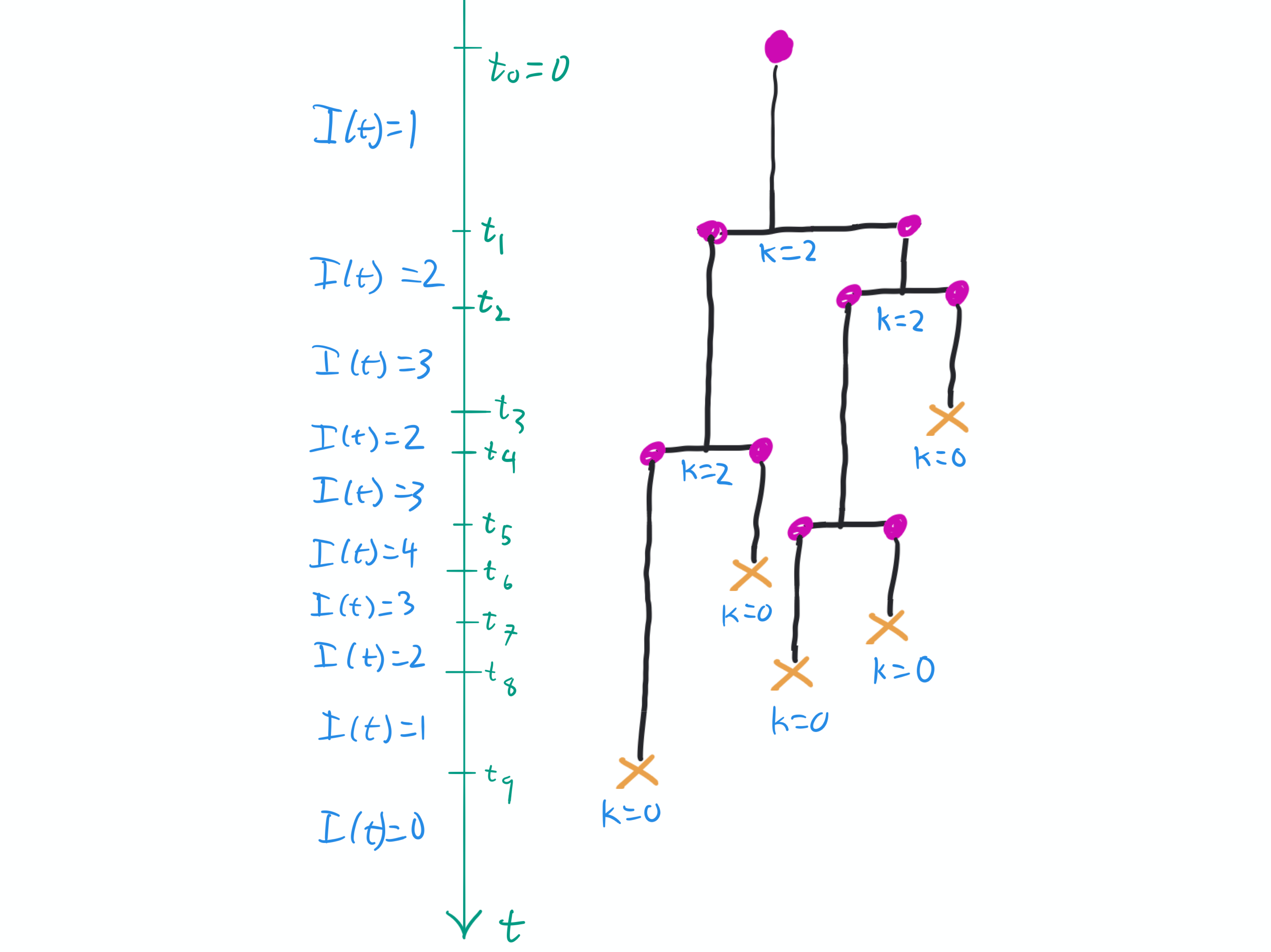
../../_images/BinaryTreeWithTime.png — Fig. 4.1 A sample illustration of $I(t)$ for a small outbreak (which could be SIS or SIR), using a Galton-Watson conceptualization. Each node persists for an exponentially distributed random time with rate $\beta+\gamma$. At that point she is replaced by either $k=0$ (crosses) or $k=2$ nodes with identical properties. The corresponding probabilities are $p_0=\gamma/(\beta+\gamma)$ and $p_2=\beta/(\beta+\gamma)$. In the disease conceptualization, the $k=0$ case corresponds to recovery. The $k=2$ case corresponds to the infected individual infecting another individual, with the same individual represented by different nodes before and after the event (we can think of the original infected individual being the left offspring and the newly infected individual being the right offspring). Although this plot shows $9$ nodes, it corresponds to exactly $5$ total individuals.#

We can convert this outbreak to a different representation which is simpler to analyze (but loses the time dependence):

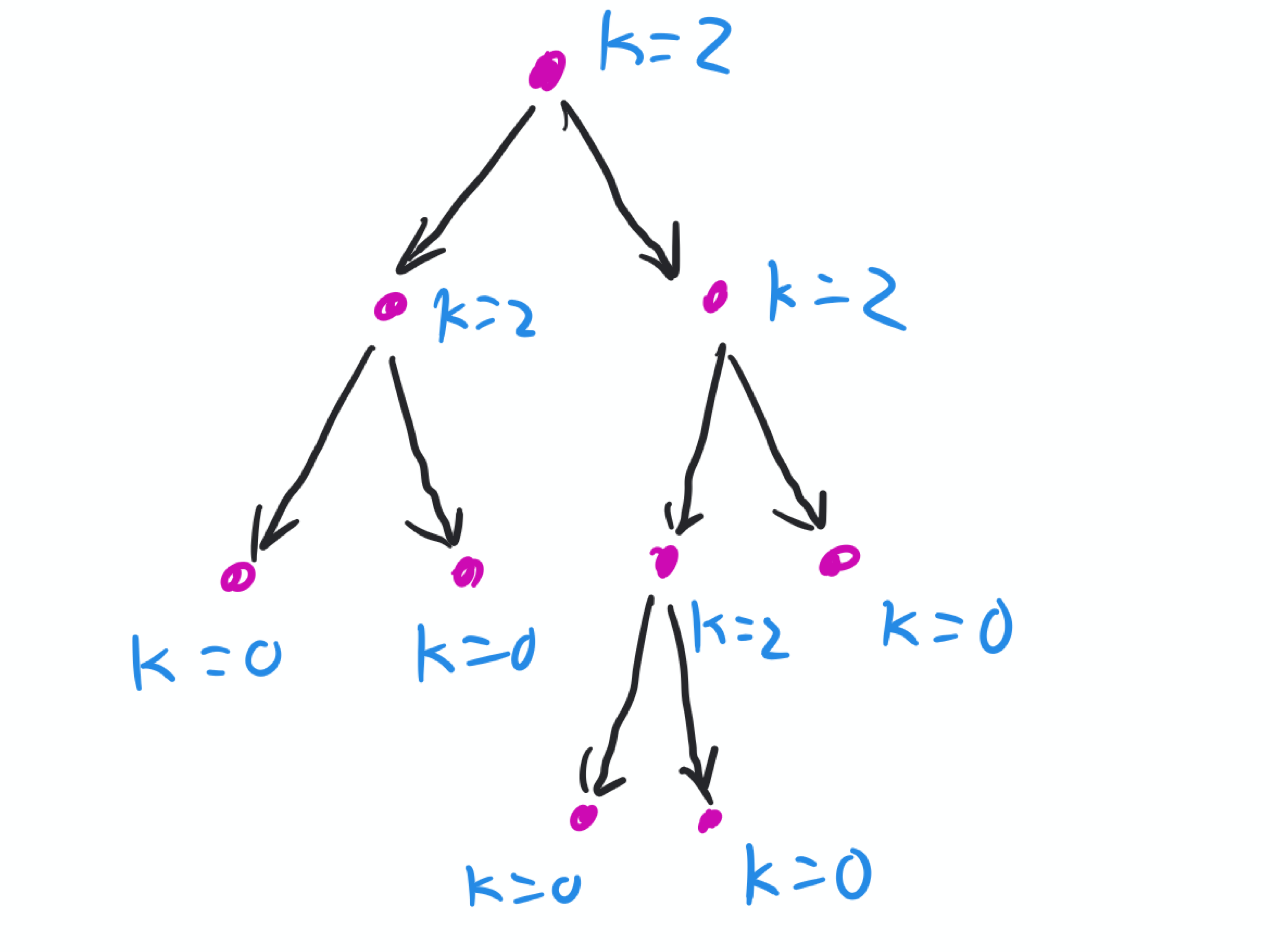
../../_images/BinaryTreeNoTime.png — Fig. 4.2 The same outbreak as in Fig. 4.1, but without the time dependence. The number of offspring of each node is more clearly visible. Again, an individual in the disease model may be represented by multiple nodes in this Galtonrepresentation.#

To determine the probability of a particular size, we will want to calculate the probability of a tree like in Fig. 4.2. To determine this probability, we first look for properties of the tree.

The following properties are relatively easy to confirm:

Each node in the Galton-Watson process has either $k=0$ or $k=2$ offspring.
Aside from the initial node, each node has a single parent.
The total number of nodes with $k=0$ corresponds to the total number of individuals infected (each infected individual eventually recovers exactly once).

If the total number of nodes in the tree is $j$, then from the fact that all nodes except the first have a single parent, we conclude that the total number of parent-offspring pairs is $j-1$. However, this is also the sum $\sum k_i$. So $\sum k_i = j-1$. There are $\frac{j-1}{2}$ nodes with $2$ offspring, so the total number of infections is $j - \frac{j-1}{2} = \frac{j+1}{2}$.

We do not yet have enough information to calculate the probability of Fig. 4.2. We will need an additional constraint. To find this constraint, we first convert the tree into a sequence of $k_i$, then we will analyze the probability of that sequence. There are two natural ways to order the nodes in Fig. 4.2, shown in Fig. 4.3.

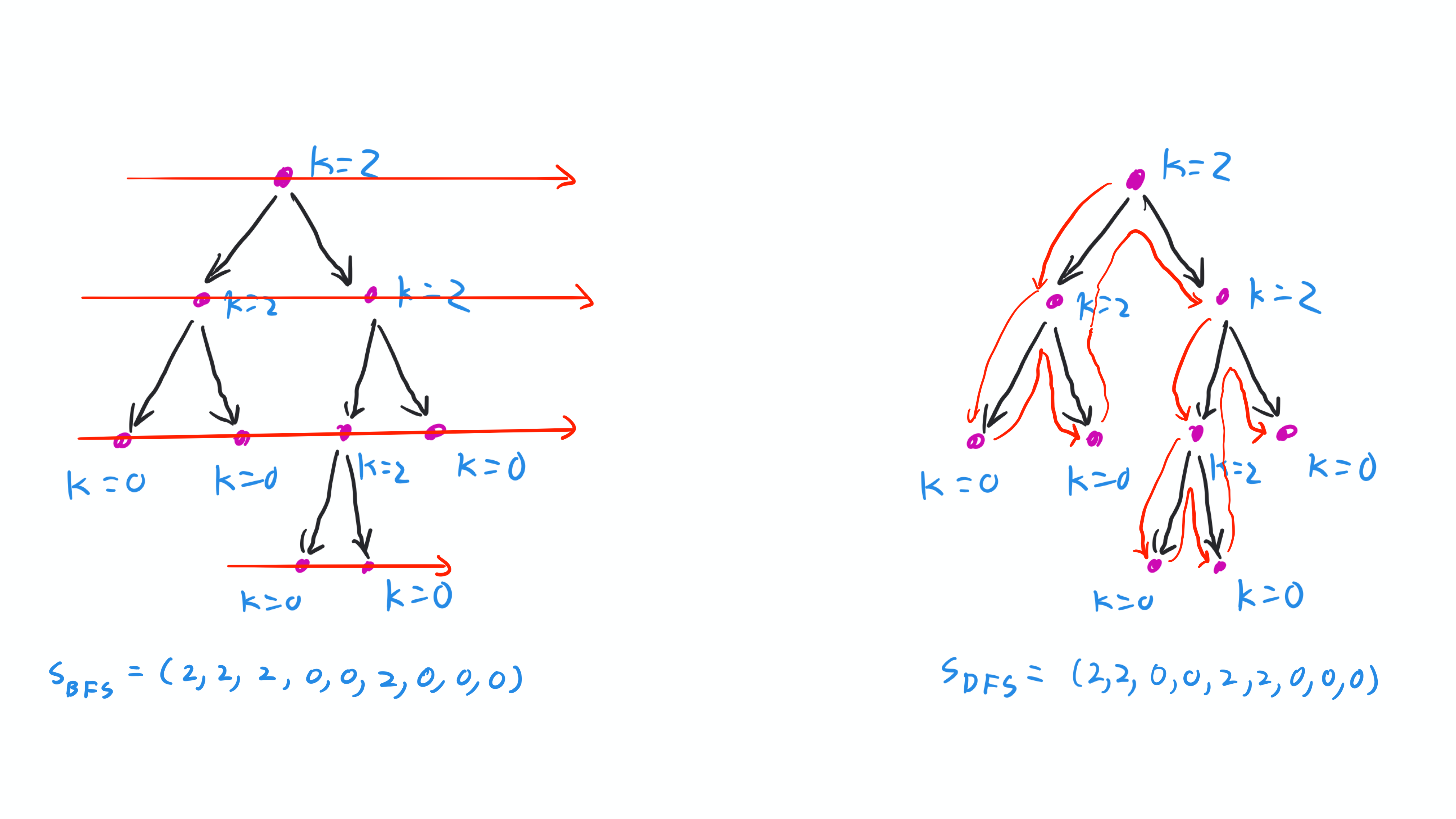
../../_images/BinaryTreeBFSvsDFS.png — Fig. 4.3 The difference between Breadth-First-Search (BFS – **Left**) and Depth-First-Search (DFS – **Right**) in a tree. In BFS we start from a node and find all nodes distance $1$, then all nodes distance $2$, etc. Each time we encounter a node, we record its degree. In DFS we first travel down one branch recursively, “exhausting” each branch before looking at the next branch.#

Many people more naturally consider Breadth-First-Search (BFS). However, for us it will be useful to use Depth-First-Search (DFS). DFS can be considered similarly to how we might expect inheritance to travel in a Royal Family in Europe. The king’s first son has priority, and that son’s sons come next, etc. So long as there is at least one son along that branch of the family tree, the king’s second son is not considered.

The advantage for this in the proof we will be doing later is that in DFS, the offspring of a node immediately follow that node in the list. In BFS, the location of a node’s offspring in the list depends on what happens in other parts of the tree. It will be much easier to reconstruct a tree from its sequence of offspring counts in the DFS case than in the BFS case.

The sequence of offspring counts in the DFS case is called a Łukasiewicz word:

Definition 4.4 (Łukasiewicz word.)

If we find a list of nodes $v_1, \ldots, v_j$ through a Depth-First search of a Galton-Watson tree, then the sequence $\mathcal{S}=k_1, \ldots, k_j$ where $k_i$ is the number of offspring of $v_i$ is called a Łukasiewicz word.

4.4.1. The Cycle Lemma#

An important part of our proof is the Cycle Lemma. Before giving it, we must define a cyclic permutation:

Definition 4.5 (Cyclic Permutation)

Given a sequence $\mathcal{S} = (s_1, s_2, \ldots, s_j)$, the $j$ cyclic permutations of $\mathcal{S}$ are:

\[\begin{align*} &(s_1, s_2, \ldots, s_j)\\ &(s_2, s_3, \ldots, s_j, s_1)\\ &(s_3, s_4, \ldots, s_j, s_1, s_2)\\ & \vdots\\ & (s_j, s_1, s_2, \ldots, s_{j-1}) \end{align*}\]

Now we are ready to give the Cycle Lemma:

Lemma 4.1 (Cycle Lemma)

Given a sequence $S$ of $j$ non-negative integers summing to $j-1$, there is a unique tree whose Łukasiewicz word is one of the cyclic permutations of $S$.

Remark 4.2

Note that in the trees above, $k$ was restricted to $0$ or $2$, but the cycle lemma does not have this restriction.

The proof will proceed by induction and create the unique tree whose Łukasiewicz word is a cyclic permutation of $S$. I am giving two related proofs, both of which are based on algoriths that reconstruct the unique three. The first is the way I set this up originally when I developed this proof. I think the second approach may be more intuitive. Both of them result in the same tree (because there is only one tree possible), but it is perhaps more obvious that the second algorithm really has no alternative outcome.

4.4.1.1. First proof#

Algorithm 4.2 (Constructing a tree from $S$)

Input

A length-$j$ sequence $S$ of non-negative integers summing to $j-1$

Output

The unique tree whose Łukasiewicz word is a cyclic permutation of $S$

Steps

Place $j$ nodes $u_1$, $u_2$, $\ldots$, $u_j$ clockwise around a circle with $u_1$ at the top.
Label each $u_i$ with $s_i$.
Repeat the following steps as long as more than one node remains:

(i) Identify a pair of adjacent nodes so that the first has $s_m>0$ and the following node has label equal to $s_n=0$ There may be multiple such pairs, the choice is arbitrary.

(ii) Add an edge from $u_m$ to $u_n$. Remove $u_n$ from the cycle, and reduce $s_m$ by $1$.

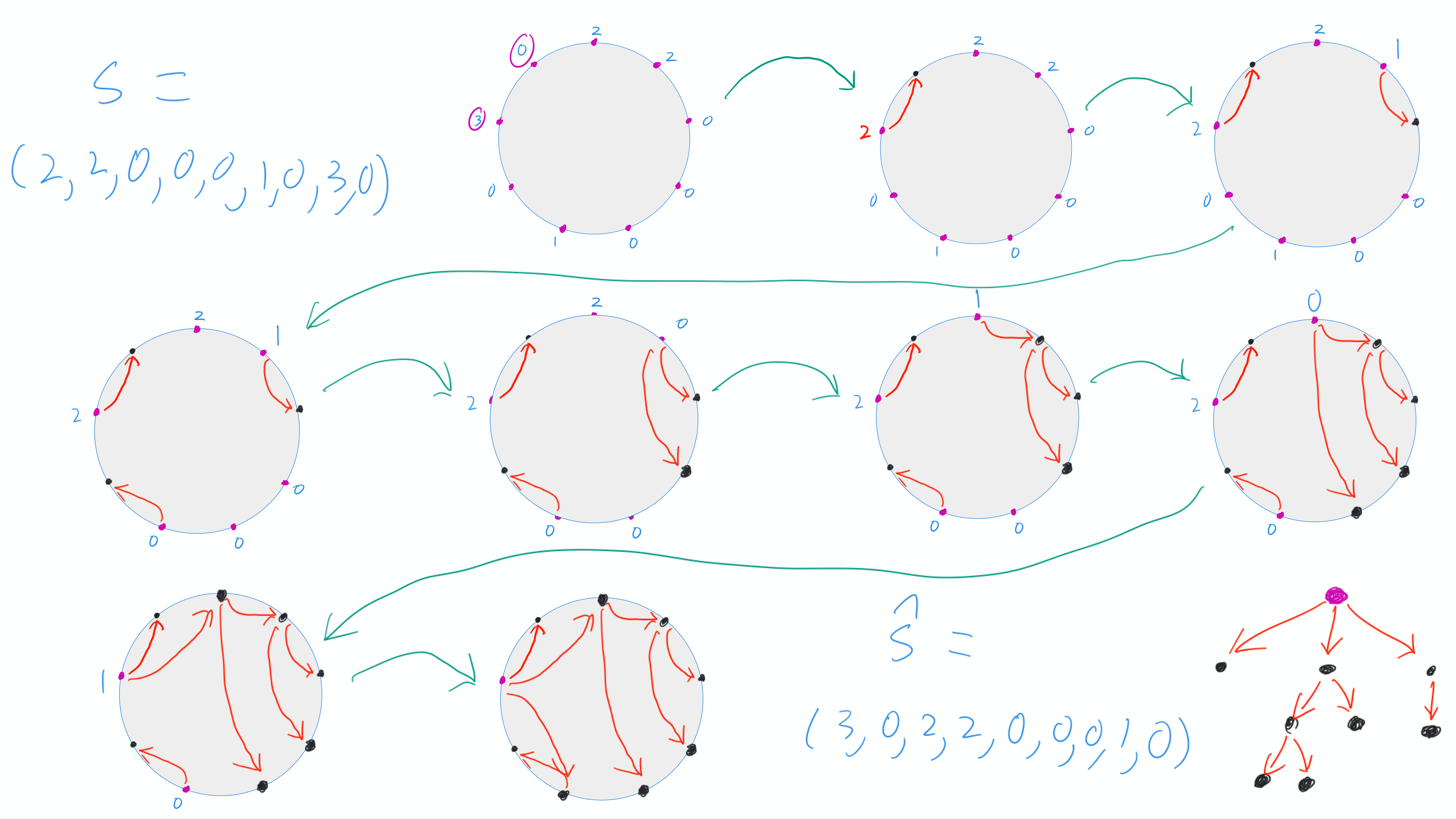
../../_images/CycleLemAlg.png — Fig. 4.4 An illustration of the steps of the algorithm. The algorithm begins with the sequence $S=(2,2,0,0,0,1,0,3,0)$. After adding an edge from a node ($u_8$) with positive label to a node ($u_9$) with zero label, a new shorter sequence $(2,2,0,0,0,1,0,2)$ emerges. Repeated steps results in a tree, but the root of the tree is not $u_1$, but rather $u_8$. Taking the cyclic permutation of the sequence that begins at the root of the tree results in a Łukasiewicz word. The choice of which $u_m$, $u_n$ pair to consider at any step is arbitrary as long as $u_n$ immediately follows $u_m$ at the current step, $s_m>0$, and $s_n=0$.#

Each step of the algorithm reduces the total number of nodes in the cycle by $1$ and reduces the sum of the $s_i$ by $1$. Thus the sum is always one less than the number of nodes. This gurantees that there is always a pair of nodes for step (3.i) until only one node remains.

Proof. Consider a length-$j$ sequence $S = (s_1, s_2, \ldots, s_j)$ of non-negative integers that sum to $j-1$.

We will use induction on $j$. If $j=1$, then $S=(0)$. This is a Łukasiewicz word, and the corresponding tree is simply the isolated node $u_1$ with no offspring.

Now consider $j \geq 2$. Place the nodes in a cycle and label them following the first two steps of Algorithm 4.2. We will prove that there is a unique tree that can be constructed with the nodes on this cycle whose ordering corresponds to a Depth-First-Search (starting from whichever node ends up being the root).

The $s_i$ sum to $j-1$ and are all non-negative integers. Because $0 < j-1< j$, we are guaranteed at least one value of $0$ and one non-zero value. It follows that somewhere there is a non-zero value $s_i>0$ which is followed immediately by $s_{i+1}=0$, (taking indices to be modulo $j$ so that if $i=j$ then $s_{j+1}=s_1$).

No matter what cyclic permutation of $S$ we consider, if it is a Łukasiewicz word there must be an edge from $u_i$ to $u_{i+1}$. Add an edge from $u_i$ to $u_{i+1}$.

Consider now the new sequence $\hat{S} = (s_1, \ldots, s_{i-1}, s_i-1, s_{i+1}, \ldots, s_j)$, which has length $j-1$ and sum $j-2$. By the inductive hypothesis, there is a unique tree on the $j-1$ nodes whose Łukasiewicz word is a cyclic permutation of $\hat{S}$, and this tree is constructed by Algorithm 4.2. Add the edges of this tree. Along with the $u_i$ to $u_{i+1}$ edge, we have a new tree with $j-1$ edges and $j$ nodes. This tree is the only possible tree constructed with this cyclic orientation.

We find the (unique) root of this tree $u_\ell$, and create the sequence $(s_\ell, s_{\ell+1}, \ldots, s_j, s_1, \ldots, s_{\ell-1})$. This is a cyclic permutation of $S$ and it is a Łukasiewicz word.

4.4.1.2. Second proof#

We provide a second algorithm to reconstruct the tree. It lays out the nodes in the same way, but goes about the construction differently. I think with this algorithm it is more obvious that this algorithm must produce a tree and that there is only one tree that can be created.

Algorithm 4.3 (Equivalent Algorithm for constructing a tree from $S$)

Input

A length-$j$ sequence $S$ of non-negative integers summing to $j-1$

Output

The unique tree whose Łukasiewicz word is a cyclic permutation of $S$

Steps

Place $j$ nodes $u_1$, $u_2$, $\ldots$, $u_j$ clockwise around a circle with $u_1$ at the top (as in Algorithm 4.2).
Label each $u_i$ with $s_i$.
Repeat the following steps as long as more than one node remains:

(i) Choose the first node (clockwise from top) with a nonzero label $s_i$.

(ii) Fill in the descendents of $u_i$ from the nodes following it in the clockwise direction. The sequence of $s_m$ going clockwise from $u_i$ must correspond to a Depth-First-Search.

Step (ii) will terminate once all of the descendents of $u_i$ have been added to the tree. This occurs the at the first $n$ such that $n$ nodes (including $u_i$) have been added for which the sum of $n$ values $s_m$ is $n-1$.

(iii) Replace $s_i$ with $0$ (representing the fact that there are $0$ additional offspring to add to it) and remove all descendents of $u_i$ from the cycle.
Once step (3) is complete, all “parent”-“offspring” edges will have been created. We put the subtrees created in each pass through (3.ii) into their appropriate positions to complete the final tree.

(note, in hindsight, orienting everything counter-clockwise would make the ordering of offspring more consistent with a natural left to right ordering, but I don’t want to make any changes after showing this to students.)

Note that the list of nodes after replacing $s_i$ with $0$ and removing all descendents of $u_i$ from the cycle preserves the property that the number remaining in the cycle is one more than the sum of the labels. This guarantees that until only one node remains it is possible to find a node with a positive value.

Example 4.1 (Demonstration of Algorithm 4.3)

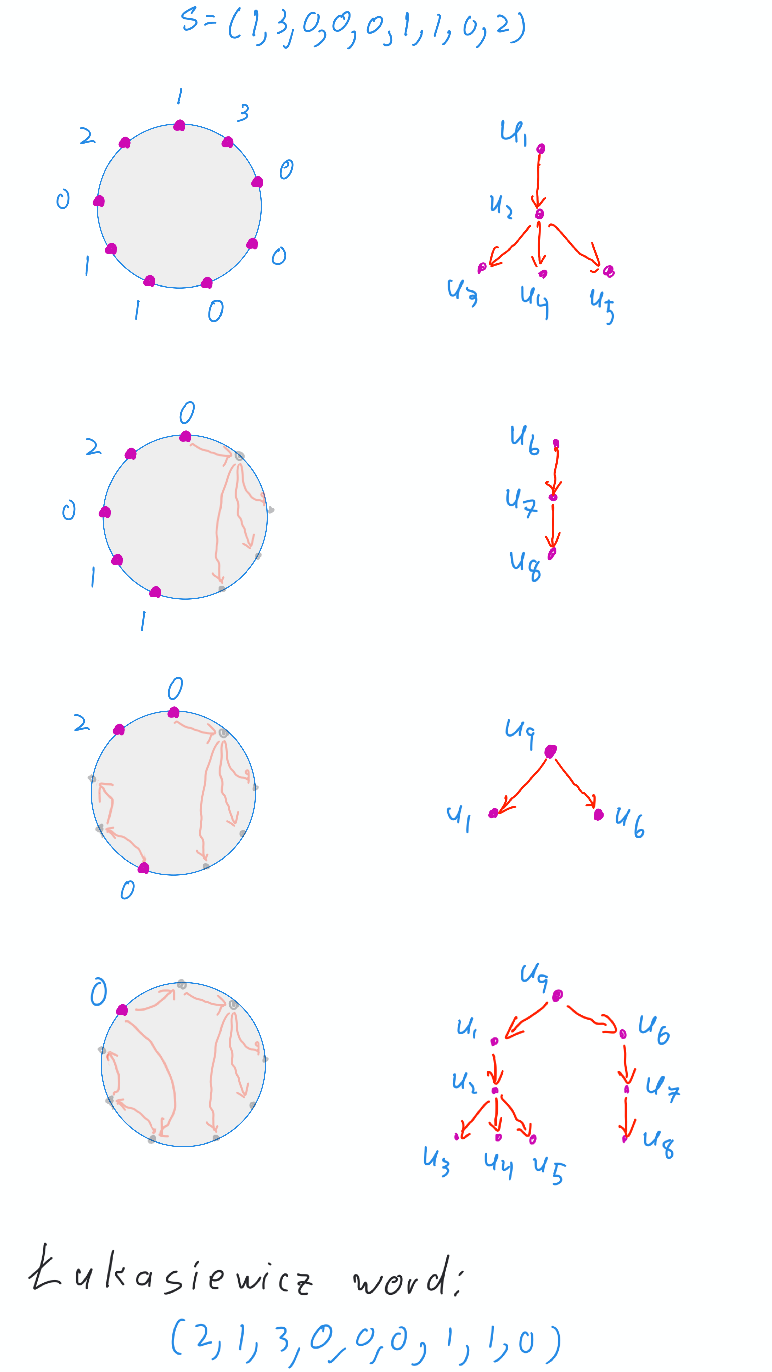
../../_images/GenerateTreeAlt.png — Fig. 4.5 The steps of the Algorithm applied to $S = (1,3,0,0,0,1,1,0,2)$.#

Consider the sequence $S = (1,3, 0,0,0, 1, 1, 0, 2)$. We put the nodes around a cycle, labelled by their offspring counts.

We are now ready to do the repetitive steps in (3).

The first nonzero entry is the first node.
After the first pass, the entire branch descending from node $u_1$ has been constructed. The sequence of the remaining nodes is $\hat{S} = (0, 1, 1, 0, 2)$.
After the second pass, the new sequence is $\hat{\hat{S}} = (0, 2, 0)$.
After the thrid pass, the sequence is $\hat{\hat{\hat{S}}}=(0)$.

The process is finished, and the remaining node is the root of the resulting tree. In this case it is the sixth node of the original sequence. We can construct the Łukasiewicz word $(2, 1, 3, 0, 0, 0, 1, 1, 0)$.

Proof. Short proof based on Algorithm 4.3

We show that if the sum of $S$ is one less than its length, then of all of the cyclic permutations of $S$, there is exactly one that is the Łukasiewicz word of a tree, and that tree is unique.

We prove by induction on $j$, the length of $S$. If we have a sequence with $j=1$ and $\sum_i s_i = 0$, then $S = (0)$ is the sequence and the single node is a unique tree.

If $j>1$, then there is a positive $s_i$ somewhere, and the algorithm can proceed. On the first pass through, it finds a node $u_i$ with at least one offspring. It creates a sub-tree of nodes that descends from $u_i$. Given the properties of depth-first-searches, the ordering of these labels after $s_i$ uniquely determines the structure of that sub-tree. That is, there is no freedom in how these nodes are joined – whether by this algorithm or by any other method – this exact subtree must end up descending from $u_i$.

When we remove the descendents’ labels from the cycle and reduce $s_i$ to $0$, the labels in the new cycle have the property that they sum to one less than the number of labels. So by induction[1] we can assume that there is exactly one cyclic permutation of these labels that is the Łukasiewicz word of a tree, and that tree is unique.

We can assume the tree on these remaining labels has been constructed and then add the descendents of $u_i$ under $u_i$. The resulting tree has a Łukasiewicz word that is a cyclic permutation of the original sequence $S$. This completes the rigorous proof.

In practice rather than calling to “induction” at the final step, we repeat the algorithm until it is complete. We may construct multiple sub-trees before we finally arrive at the root and then construct the entire tree.

I recommend that you consider what happens if you take the original sequence in Example 4.1, and start the algorithm from the beginning, except that in step (3) you use the root node as the starting point. You should see that every time you generate the subtree descending from any one node, there is no freedom at all. If you don’t start at the root, you simply construct a subtree of the entire tree.

4.4.2. Finding the probability that a Galton-Watson tree has $j$ nodes#

We consider a Galton-Watson tree as above with $p_0 = \frac{\gamma}{\beta+\gamma}$ and $p_2 = \frac{\beta}{\beta+\gamma}$. When we construct the Łukasiewicz word, at each stage the probability that the next node has $k=0$ or $k=2$ is an independent choice with probabilities $p_0$ and $p_2$. This means that the probability of a tree with a specific length-$j$ Łukasiewicz word is equal to the probability that a length-$j$ sequence of values chosen independently from the offspring distribution is that Łukasiewicz word.

The probability that a Galton-Watson process will terminate after exactly $j$ nodes is equal to the sum of the probabilities of all such trees. This in turn is equal to the sum of the probabilities of each Łukasiewicz word. In other words,

\[\begin{align*} \mathbb{P}\left[\begin{array}{c} \text{Process ends with}\\[-1ex] \text{exactly $j$ nodes}\end{array}\right] &= \sum_{\begin{array}{c}\text{trees with}\\[-1ex] \text{$j$ nodes}\end{array}} \mathbb{P}[\text{tree}]\\ &= \sum_{\begin{array}{c}\text{trees with}\\[-1ex] \text{$j$ nodes}\end{array}} \mathbb{P}[\text{Łukasiewicz word of tree}]\\ \end{align*}\]

We don’t have a direct way to sum the probabilities of the Łukasiewicz words. However, we do have a way to calculate the probability that a sequence of $j$ numbers sums to $j-1$ (it is $[x^{j-1}]\hat{\mu}(x)^j$). We now find a way to express the sum of the probabilities of the Łukasiewicz words in terms of this.

Consider a Łukasiewicz word and all of its cyclic permutations. Call this the orbit of the Łukasiewicz word. The cycle lemma says that each length-$j$ sequence that sums to $j-1$ is in the orbit of exactly one Łukasiewicz word. Or in other words, the orbits of Łukasiewicz words exactly partition the set of length-$j$ sequences that sum to $j-1$. This gives hope that we can find the combined probability of the Łukasiewicz words in terms of the known probability that a length-$j$ sequence sums to $j-1$.

Because each sequence in the orbit has the same numbers in it (just in a different order), they all have the same probability. Thus the probability a randomly-generated sequence is in the orbit of a given Łukasiewicz word is equal to $j$ times the probability of that Łukasiewicz word. Or, equivalently, the probability of a given Łukasiewicz word is equal to $1/j$ times the combined probability of all the sequences in its orbit. We now have

\[\begin{align*} \mathbb{P}\left[\begin{array}{c} \text{Process ends with}\\[-1ex] \text{exactly $j$ nodes}\end{array}\right] &=\sum_{\begin{array}{c} \text{trees with}\\[-1ex] \text{$j$ nodes}\end{array}} \mathbb{P}[\text{Łukasiewicz word of tree}]\\ &= \sum_{\begin{array}{c} \text{trees with}\\[-1ex] \text{$j$ nodes}\end{array}} \frac{1}{j} \mathbb{P}\left[\begin{array}{c} \text{a random length-$j$ sequence is in}\\[-1ex] \text{orbit of Łukasiewicz word of tree} \end{array}\right] \end{align*}\]

We now do some Algebra and use the fact that the orbits of Łukasiewicz words form a partition of the set of length-$j$ sequences that sum to $j-1$. We first change our sums to be over the Łukasiewicz words rather than over the trees.

\[\begin{align*} \mathbb{P}\left[\begin{array}{c} \text{Process ends with}\\[-1ex] \text{exactly $j$ nodes}\end{array}\right] &= \frac{1}{j} \sum_{\begin{array}{c}\text{length $j$}\\[-1ex] \text{Łukasiewicz words}\end{array}} \mathbb{P}\left[\begin{array}{c} \text{a random length-$j$ sequence is in} \\[-1ex] \text{the orbit of the Łukasiewicz word}\end{array}\right]\\ &= \frac{1}{j} \mathbb{P}\left[\begin{array}{c}\text{a random length-$j$ sequence is in}\\[-1ex] \text{the orbit of some Łukasiewicz word}\end{array}\right]\\ &= \frac{1}{j} \mathbb{P}\left[\begin{array}{c} \text{a random length-$j$ sequence}\\[-1ex] \text{sums to $j-1$} \end{array}\right] \end{align*}\]

To get the second line, we used the law of total probability.
To get the third line we used the fact that a length-$j$ sequence sums to $j-1$ iff it is in the orbit of a Łukasiewicz word which means

\[\begin{split} \left\{ \begin{array}{c}\text{length-$j$ sequences in the}\\[-1ex] \text{orbit of some Łukasiewicz word}\end{array} \right\} = \left\{ \begin{array}{c} \text{length-$j$ sequences}\\[-1ex] \text{that sum to $j-1$} \end{array} \right\} \end{split}\]

Since the sets are the same, their probabilities are the same.

Now consider the set of all length-$j$ sequences that satisfy the constraint of summing to $j-1$. This has combined probability $[x^{j-1}]\hat{\mu}(x)^j$ by Corollary 1.2 (this is the step that justifies including this result in a subject on PGFs).

Thus we have

\[\begin{align*} \mathbb{P}\left[\begin{array}{c} \text{Process ends with}\\[-1ex] \text{exactly $j$ nodes}\end{array}\right] &=\frac{1}{j} \mathbb{P}\left[\begin{array}{c}\text{a random length-$j$}\\[-1ex] \text{sequence sums to $j-1$}\end{array}\right]\\ &= \frac{1}{j} \left[x^{j-1}\right]\left(\hat{\mu}(x)^j\right) \end{align*}\]

We’re now done with the major ideas of the proof. From this point on, the ramaining steps are effectively just doing algebra to convert the probability of $j$ nodes to the probability of $\ell$ infections. We have already noted that if there are $j$ nodes in the tree as constructed, then the number of infections in the SIS or SIR process is $\ell = (j+1)/2$. We first calculate the probability of $j$ nodes using $\hat{\mu}(x) = \frac{\gamma}{\beta+\gamma} + \frac{\beta}{\beta+\gamma}x^2$:

\[\begin{align*} \mathbb{P}\left[\begin{array}{c} \text{Process ends with}\\[-1ex] \text{exactly $j$ nodes}\end{array}\right] &= \frac{1}{j} \left[x^{j-1}\right]\big( \hat{\mu}(x)^j\big)\\ &= \frac{1}{j} \left[x^{j-1}\right] \left(\left(\frac{\gamma}{\beta+\gamma} + \frac{\beta}{\beta+\gamma} x^2 \right)^j\right)\\ &= \frac{1}{j} \left[x^{j-1}\right] \sum_{k=0}^j \binom{j}{k} \frac{\gamma^k}{(\beta+\gamma)^k} \frac{\beta^{j-k} x^{2(j-k)}}{(\beta+\gamma)^{j-k}}\\ &= \frac{1}{j} \frac{1}{(\beta+\gamma)^j}\left[x^{j-1}\right] \sum_{k=0}^j \binom{j}{k} \gamma^k\beta^{j-k}x^{2(j-k)}\\ &= \begin{cases} \frac{1}{j} \frac{1}{(\beta+\gamma)^j} \binom{j}{\frac{j+1}{2}} \gamma^{(j+1)/2}\beta^{(j-1)/2} & j \text{ odd}\\[1ex] 0 & j \text{ even} \end{cases} \end{align*}\]

Since $\ell = (j+1)/2$ is the total number of individuals infected, we conclude that the probability of $\ell$ infections is

\[\begin{align*} \mathbb{P}[\ell \text{ infections}] &= \frac{1}{2\ell-1} \frac{1}{(\beta+\gamma)^{2\ell-1}} \binom{2\ell-1}{\ell} \gamma^\ell \beta^{\ell-1}\\ &= \frac{\gamma^\ell \beta^{\ell-1}}{(\beta+\gamma)^{2\ell-1}} \frac{1}{2\ell-1}\frac{(2\ell-1)!}{\ell! (\ell-1)!}\\ &= \frac{\gamma^\ell \beta^{\ell-1}}{(\beta+\gamma)^{2\ell-1}}\frac{1}{\ell} \frac{(2\ell-2)!}{(\ell-1)! (\ell-1)!}\\ &=\frac{\gamma^\ell \beta^{\ell-1}}{(\beta+\gamma)^{2\ell-1}} \frac{1}{\ell}\binom{2\ell-2}{\ell-1}\\ &= \frac{1}{\ell}\frac{\gamma^\ell \beta^{\ell-1}}{\gamma^{2\ell-1}(\beta/\gamma+1)^{2\ell-1}} \binom{2\ell-2}{\ell-1}\\ &= \frac{1}{\ell}\frac{\mathcal{R}_0^{\ell-1}}{(\mathcal{R}_0+1)^{2\ell-1}} \binom{2\ell-2}{\ell-1} \end{align*}\]

where we introduced the variable $\mathcal{R}_0 = \beta/\gamma$.

It’s natural to wonder why I converted $\frac{1}{2\ell-1} \binom{2\ell-1}{\ell}$ to $\frac{1}{\ell} \binom{2\ell-2}{\ell-1}$. I did this because I’ve looked ahead at the more general formula we will see when we look at a “generation-based” perspective and the connections are more obvious if it is written this way.

We have proven:

Theorem 4.2 (Continuous-time SIS and SIR small outbreak size distribution)

Consider the SIS and SIR disease models with transmission rate $\beta$ and recovery rate $\gamma$ and $\mathcal{R}_0 = \beta/\gamma$. In the $N \to \infty$ limit, the probability an outbreak ends with exactly $\ell$ infections is

\[ \mathbb{P}[\ell \text{ infections}]=\frac{1}{\ell}\frac{\mathcal{R}_0^{\ell-1}}{(\mathcal{R}_0+1)^{2\ell-1}} \binom{2\ell-2}{\ell-1} \]

Example 4.2 (Small Outbreak Size Distribution if $\beta = 3\gamma/2$)

If $\beta = 3 \gamma/2$ as in the simulations performed in earlier sections, then

\[\begin{align*} \mathbb{P}[\ell \text{ infections}] &= \frac{1}{\ell}\frac{(3/2)^{\ell-1}}{(5/2)^{2\ell-1}} \binom{2\ell-2}{\ell-1}\\ \end{align*}\]

This leads to

Size	Probability
$1$	$2/5 = 0.4$
$2$	$12/125 =0.096$
$3$	$3^2 2^4/5^5 = 0.04608$

4.4.3. Self-test#

Consider $S = (1, 0, 0, 2, 1)$ use both algorithms to construct a tree and find the Łukasiewicz word. Verify that the Łukasiewicz word is a cyclic permutation of $S$.
Now consider the first proof and first algorithm of the Cycle Lemma. Take $S = (1,0,0,3,0,1)$. By looking at the $(3,0)$ pair and your answer to (1), perform the inductive step of the proof. That is, consider the sequence after adding the edge for the $(3,0)$ pair. Match this with your answer to (1) and then update your tree to include this edge. Verify that the Łukasiewicz word is a cyclic permutation of $S$.
Now consider the second proof and algorithm for the Cycle Lemma. Take $S = (2,1,0,0,1,1,0,0,3)$. After the first step, this should be a cyclic permuation of the sequence in (1). Starting with your tree for (1), do the inductive step of the second proof to create the tree. Verify that the Łukasiewicz word is a cyclic permutation of $S$.
Consider the offspring distribution PGF $\hat{\mu}(x)=0.25 + 0.75x^2$. We will revisit the derivation of the probability of trees of size $j$ (assuming the cycle lemma is already proven). We will consider the case $j=5$.

(a) Write out all length-$5$ sequences made up of $0$ and $2$ and sum up to $4$.

(b) Group this set of sequences into orbits of cyclic permutations.

(c) For each orbit, find the Łukasiewicz word.

(d) In this case each such sequence has the same probability. Calculate this probability.

(e) Confirm that the probability of each Łukasiewicz word is $1/5$ times the probability of its orbit.

(f) Confirm that the probability of all of the Łukasiewicz word sequences is $(1/5) [x^4]\hat{\mu}(x)^5$.
Revisit (4), but this time with length-$4$ sequences that sum to $3$ where we have $\mu(x) = 1/4 + x/4 + 2x^2/4$. You should see that the sequences do not all have the same probabilities.

(a) Write out all length-$4$ sequences made up of $0$, $1$, and/or $2$ and sum up to $3$. (there are 16 such sequences)

(b) Group this set of sequences into orbits of cyclic permutations.

(c) For each orbit, find the Łukasiewicz word.

(d) For each orbit, find the probability of the sequences.

(e) Confirm that the probability of each Łukasiewicz word is $1/4$ times the probability of all of the sequences in its orbit.

(f) Confirm that the probability of all of the Łukasiewicz word sequences is $(1/4) [x^3]\mu(x)^4$.
The proofs of the cycle lemma allow for entries that are not $0$ or $2$. However, for the continuous-time SIS and SIR model, we know that all entries are $0$ or $2$.

Imagine we restricted the lemma to sequences of just $0$ and $2$. Show that the inductive step in the first proof technique would fail, but the inductive step in the second technique would not.
Stirling’s approximation states that

\[ n! \sim \sqrt{2\pi n} \left(\frac{n}{e}\right)^n \]

(the $\sim$ means that the ratio tends to $1$ as $n \to \infty$)

(a) Use this to estimate $\frac{1}{\ell}\binom{2(\ell-1)}{\ell-1}$ for large $\ell$.

(b) If $\mathcal{R}_0=1$, estimate the probability of $\ell$ infections for large $\ell$.

(c) If $\mathcal{R}_0<1$, show that as $\ell$ grows, the probability of $\ell$ infections decays much faster than for $\mathcal{R}_0=1$.

(d) Repeat (c), but for $\mathcal{R}_0>1$.

Size	Probability
\(1\)	\(2/5 = 0.4\)
\(2\)	\(12/125 =0.096\)
\(3\)	\(3^2 2^4/5^5 = 0.04608\)

Total size distribution of Continuous-Time small outbreaks: N \to \infty

Contents

4.4. Total size distribution of Continuous-Time small outbreaks: \(N \to \infty\)#

4.4.1. The Cycle Lemma#

4.4.1.1. First proof#

4.4.1.2. Second proof#

4.4.2. Finding the probability that a Galton-Watson tree has \(j\) nodes#

4.4.3. Self-test#