

2.5. Size Distribution at Successive Generations#
Please read Section 1.7, Section 1.8, and Section 1.9 before reading this section.
The major result we rely on in this section is Theorem 1.5: if \(\mu_1(x)\) and \(\mu_2(x)\) are both PGFs, then \(\psi(x) = \mu_1(\mu_2(x))\) is the PGF for the following process: First we choose \(k\) from the distribution of \(\mu_1(x)\). Then we choose \(k\) numbers from the distribution of \(\mu_2(x)\) and add them together. That is, we are taking a sum of numbers from the distribution of \(\mu_2(x)\) and the number of terms in the sum is taken from the distribution of \(\mu_1(x)\).
We will define \(\Phi_g(x)\) to be the PGF of the distribution of \(X_g\), the total size[1] at generation \(g\). For notational purposes, we set \(q_{g,k} = \mathbb{P}[X_g=k]\) to be the probability that at generation \(g\) we have \(X_g=k\) is the size of the population. So \(\Phi_g(x) = \sum_{k=0}^\infty q_{g,k}x^k\). As \(q_{0,1}=1\), we know \(\Phi_0(x)=x\) and as \(q_{1,k}=p_k\), we know \(\Phi_1(x) = \mu(x)\).
We are interested in how to calculate \(\Phi_g(x)\) for \(g>1\). Based on our above observations we have the following theorem:
Theorem 2.3 (Galton-Watson sizes at later generations)
If \(\mu(x)\) is the PGF of the offspring distribution of a Galton-Watson process then \(\Phi_g(x)\), the PGF of the distribution of \(X_g\), satisfies
that is, \(\Phi_0(x) = x\), \(\Phi_1(x)=\mu(x)\), \(\Phi_2(x)=\mu(\mu(x))\), \(\cdots\), \(\Phi_g(x) = \mu^{(g)}(x) = \mu(\mu(\mu(\cdots \mu(x)\cdots)))\).
We will give two proofs of this theorem. At first glance the difference between the two proofs appears trivial. However, later when we will look at continuous-time variations of the Galton-Watson process the two methods will lead to very different equations (which will yield the same solution).
Proof. Forward Proof
We use induction on the generation \(g\). At the base case, \(g=0\), we know that \(X_0=1\), so \(\mathbb{P}[X_0=1]=1\) and thuas \(\Phi_0(x)=1x^1\).
For the inductive step, we know that the distribution of \(X_{g}\) is \(\Phi_{g}(x)\). By the definition of the Galton-Watson process, \(X_{g+1}\) is found by choosing \(X_{g}\) numbers from the offspring distribution and adding them together. So the PGF of the distribution of \(X_{g+1}\) is \(\Phi_{g+1}(x) = \Phi_{g}(\mu(x)) = \mu^{(g+1)}(x) = \mu(\Phi_g(x))\), \(\ldots\).
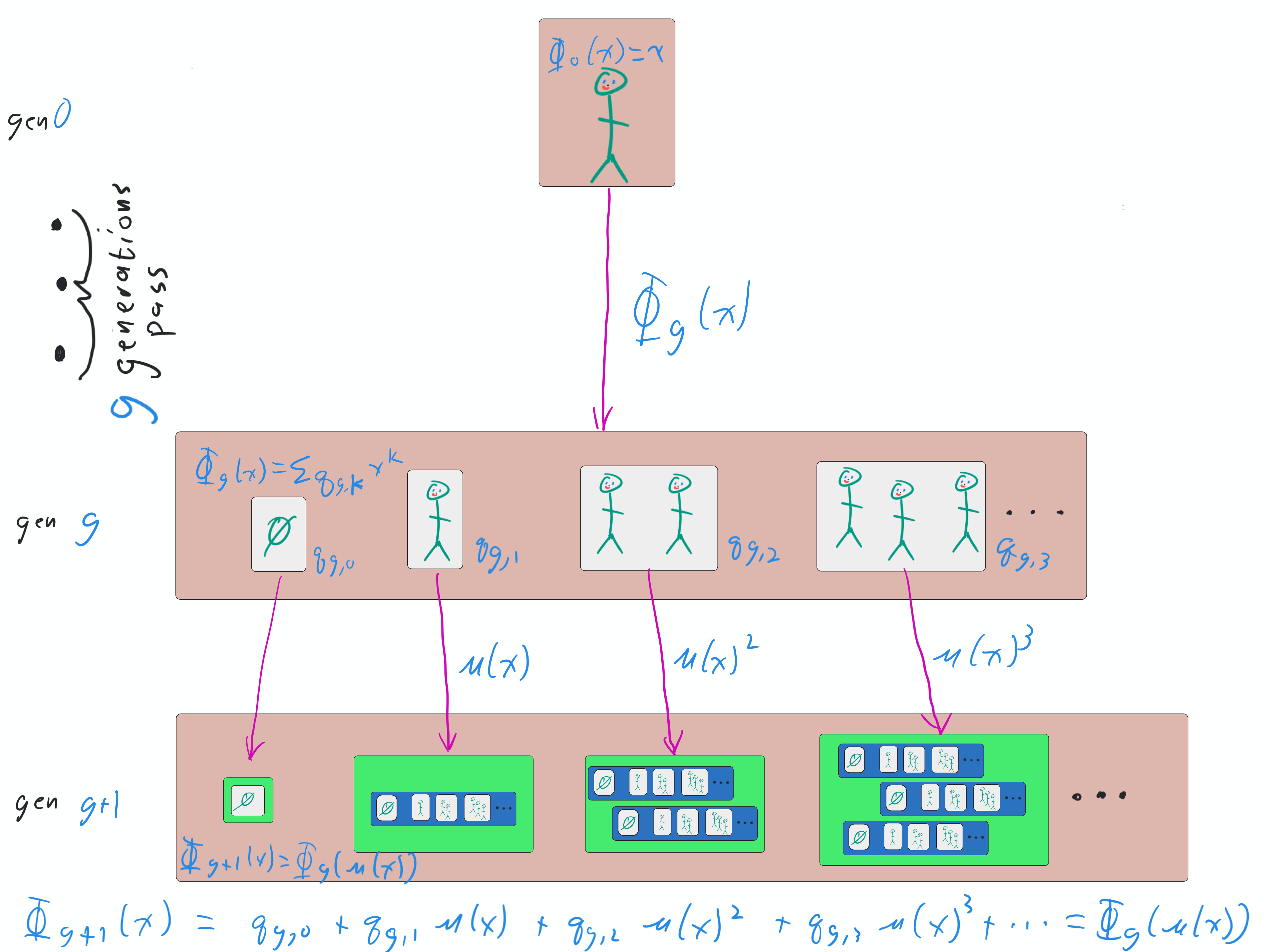
Fig. 2.4 The “forward” derivation of the PGF for \(X_g\), \(\Phi_g(x) = \sum_{k=0}^\infty q_{g,k} x^k\). By induction we can assume we know \(\Phi_g(x)\), which gives us the size distribution of generation \(g\). Each individual in generation \(g\) causes a number of offspring whose distribution has PGF \(\mu(x)\). Adding up all of these across the individuals in generation \(g\) gives \(X_{g+1}\). By Theorem 1.5, \(\Phi_{g+1}(x) = \Phi_g(\mu(x))\).#
We now show an alternate proof:
Proof. Backward Proof
We again use induction on the generation \(g\). At the base case, \(g=0\), we again know that \(X_0=1\), so as before, \(\Phi_0(x)=x\).
For the inductive step, we know that the distribution of \(X_{g}\) is \(\Phi_g(x)\). We know that chain of descendents from each individual in generation \(1\) can be thought of as the start of its own Galton-Watson process, and the number of individuals at generation \(g\) from each of the generation \(1\) individuals is \(\mu(\Phi_g(x))\).
Since the number of individuals at generation \(1\) has PGF \(\mu(x)\) and the number of descendents after \(g\) from each of these has PGF \(\Phi_g(x)\), we conclude that the size distribution at generation \(g\) has PGF \(\Phi_{g+1} = \mu(\Phi_g(x))\).
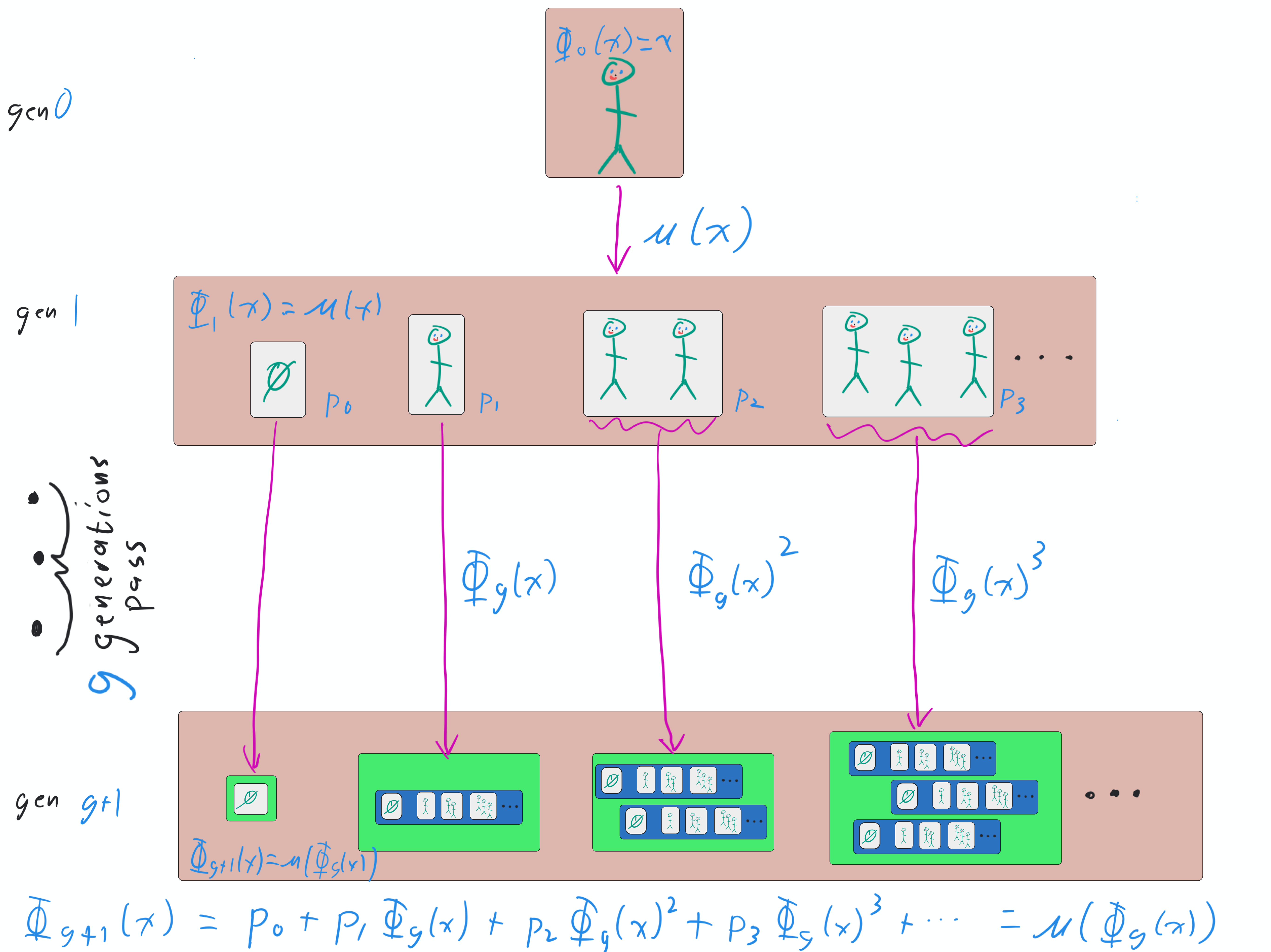
Fig. 2.5 The “backward” derivation of the PGF for \(X_g\), \(\Phi_g(x) = \sum_{k=0}^\infty q_{g,k} x^k\). We know the size distribution of generation \(1\) has PGF \(\mu(x)\). For each individual in generation \(1\), the number of descendents \(g\) generations below it has PGF \(\Phi_g(x)\) by induction. Adding up all of these across the individuals in generation \(1\) gives \(\Phi_{g+1}(x)\). By Theorem 1.5, \(\Phi_{g+1}(x) = \Phi_g(\mu(x))\).```#
2.5.1. Expected size of a Galton-Watson Process at generation \(g\)#
We have seen that the size of a Galton Watson process at generation \(g\), \(X_g\) has PGF \(\Phi_{g}(x) = \mu(\Phi_{g-1}(x))\). The average size at generation \(g\), \(\mathbb{E}[X_g]\) is given for \(g>1\) by
The fact that \(\mathbb{E}[X_g]\) can be written in terms of \(\mathbb{E}[X_{g-1}]\) strongly suggests an inductive proof of the following theorem is possible:
Theorem 2.4 (Average Size of a Galton Watson Process after \(g\) generations)
The expected size of a Galton Watson process at generation \(g\) is
The proof is given as an exercise.
2.5.2. Distribution of \(X_g\)#
Please read Section 1.10 before reading this subsection.
For each generation \(g\), our formulas above give us a way to construct \(\Phi_g(x)\), the PGF of \(X_g\). However, we will often want to know the individual coefficients \(p_{g,k}\) of \(\Phi_g(x) = \sum_k p_{g,k}x^k\).
We can find \(\Phi_0(x)= x\) and \(\Phi_1(x) = \mu(x)\) fairly easily. To find \(\Phi_2(x) = \mu(\Phi_1(x))\), it may be tempting to plug in the series expansion for \(\Phi_1(x)\) into the expansion for \(\mu(x)\) and track what happens to the coefficients. However, this can be computationally expensive (both in terms of memory and number of calculations).
In Section 1.10 we see that an alternative method to calculate the coefficients of \(\Phi_g(x)\) is through a Cauchy integral:
We can do this numerically by setting \(\theta_m = 2\pi m/M\) for \(m=0, 1, \ldots, M-1\) for some large value of \(M\), and then using Riemann integration to perform the integral.
2.5.3. Self-test#
Use Theorem 2.3 to show that the probability of extinction after \(g\) generations is \(\Phi_g(0) = \mu^{(g)}(0)\).
Use proof by induction to show that the expected size of generation \(g\) is \(\mu'(1)^g\). That is, prove that \(\phi_g'(1) = \mu'(1)^g\).
Using the two previous answers, what is the expected size of Galton-Watson processes that are not extinct by generation \(g\)?
this question is incomplete Use a case with \(\mu'(1)=1\) and explore size distribution on logscale.