

3.2. Continuous Time Galton Watson Process#
Significant edits:
22 Jan 2025: Added self-test question 4 to understand equivalence of definition
end edit description
We now assume that we begin with a single individual and individuals reproduce or die as Poisson processes. Individuals reproduce with one rate (having a possibly random number of offspring) and die with another rate.
Conceptually if all we care about is the counts at time \(t\), one individual creating \(k-1\) offspring is equivalent to one individual being removed and replaced by \(k\) offspring. This allows us to combine our reproduction and deaths into a single superposition of the Poisson processes with a combined rate \(r = \sum_k r_k\) where \(r_k\) is the probability of being replaced by \(k\) offspring.
This leads to the following definition:
Definition 3.3 (Continuous-Time Galton-Watson Process)
A continuous-time Galton-Watson process is defined as follows.
The process begins with \(X(0)=1\).
\(X\) changes by discrete jumps at time \(t_1\), \(t_2\), \(\ldots\), with the time between \(t_i\) and \(t_{i+1}\) exponentially distributed with total rate \(X(t_i) r\) (taking \(t_0=0\)).
At the jumps, \(X\) changes by an amount \(k-1\) with probability \(p_k = r_k/r\) (so \(\sum_k r_k = r < \infty\)).
We can create a definition resembling the Galton-Watson Tree definition.
Definition 3.4 (Continuous-Time Galton Watson Process)
A continuous-time Galton-Watson process is defined as follows.
The process begins with a single individual at \(t=0\).
Each individual lives for an exponentially distributed time with total rate \(r = \sum_{k\geq 0} r_k < \infty\), independently of all other events.
Upon death, she is instantaneously replaced by \(k\) individuals with probability \(r_k/r\), independently of all other events.
Using \(p_k=r_k/r\) to be the probability that after an event, the individual has been replaced by \(k\) individuals, we define
Definition 3.5 (The Offspring PGF \(\hat{\mu}(x)\))
We will use the PGF
to be the PGF of the offspring distribution in the continuous time Galton-Watson process.
Definition 3.6 (\(X(t)\) and \(\Phi(x,t)\))
We use \(X(t)\) to denote the (stochastic) population size at time \(t\) and
where \(q_k = \mathbb{P}[X(t)=k]\).
If all we care about is calculating \(X(t)\), we can assume \(p_1 \neq 0\). For most infectious disease models we will assume that only \(p_0\) and \(p_2\) are nonzero, but for other processes we can have \(p_k >0\) for \(k >2\).
Note that if we want to count the cumulative number of individuals in our real-world application, we cannot assume that the individual is removed and then replaced when giving birth. We would need to be careful with the accounting in this case.
3.2.1. Finding \(\Phi(x,T_1+T_2)\)#
To see how \(\Phi(x,t)\) changes in time, it will be important to know how to find \(\Phi(x,T_1+T_2)\) if we know \(\Phi(x,T_1)\) and \(\Phi(x,T_2)\).
This will rely heavily on our earlier result about “Randomly Stopped Sums”, Theorem 1.5. That is, if we take the sum
where \(k\) is a random number with PGF \(\mu_1(x)\) and \(m_i\) are independent random numbers with PGF \(\mu_2(x)\), then the PGF for \(X\) is \(\mu_1(\mu_2(x))\).
Lemma 3.1 (The PGF of \(\Phi(x,T_1+T_2)\))
Consider a continuous-time Galton-Watson Process with \(X(t)\) representing the (random) population size at time \(t\). Then
Proof. To prove this, we consider the image illustrated in Fig. 3.1. The size \(X(T_1+T_2)\) found by considering each of the individuals \(u_i\), \(i=1, \ldots, X(T_1)\) at time \(T_1\). We set \(m_i\) to be the number of descendents of \(u_i\) at time \(T_1+T_2\).
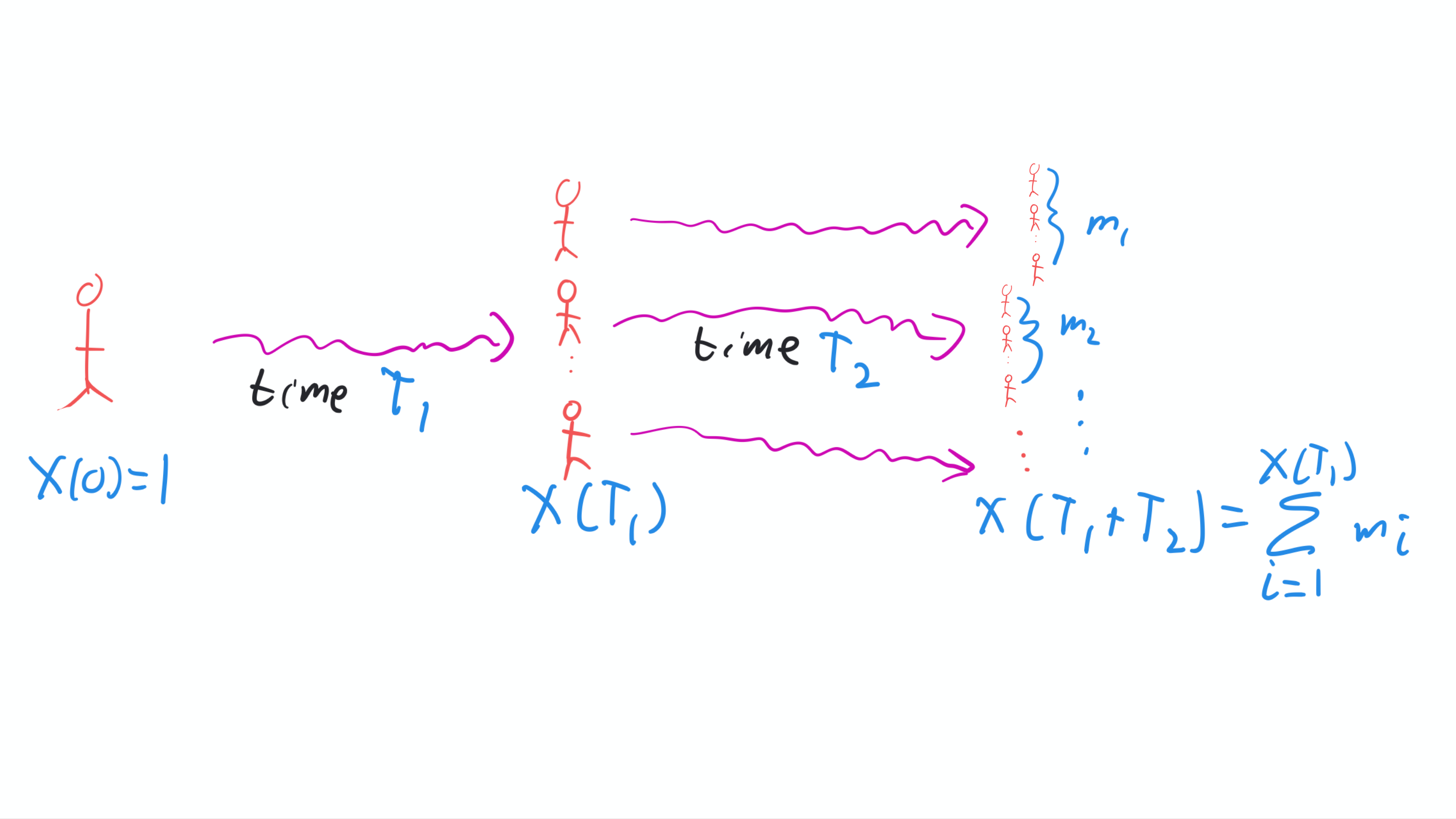
Fig. 3.1 Illustration of how \(X(T_1+T_2)\) depends on \(X(T_1)\) and the number of descendents of each individual present at time \(T_1\) has at time \(T_1+T_2\).#
So
Our key observation is that the distribution of \(X(T_2)\) does not just tell us the distribution of the number present at time \(T_2\). It is also the distribution of the result if we choose an individual at time \(t\), wait for a time period of \(T_2\) (that is, wait until \(t+T_2\)) and count its descendents. So each \(m_i\) is a random variable with the same distribution as \(X(T_2)\).
This is a randomly stopped sum. By Theorem 1.5, the PGF of \(X(T_1+T_2)\) is the PGF of \(X(T_2)\) (that is, \(\Phi(x,T_2)\)) plugged into the PGF of \(X_1\) (that is, \(\Phi(x,T_1)\)). So we have
Fig. 3.2 translates the count-based information in Fig. 3.1 into a PGF framework.
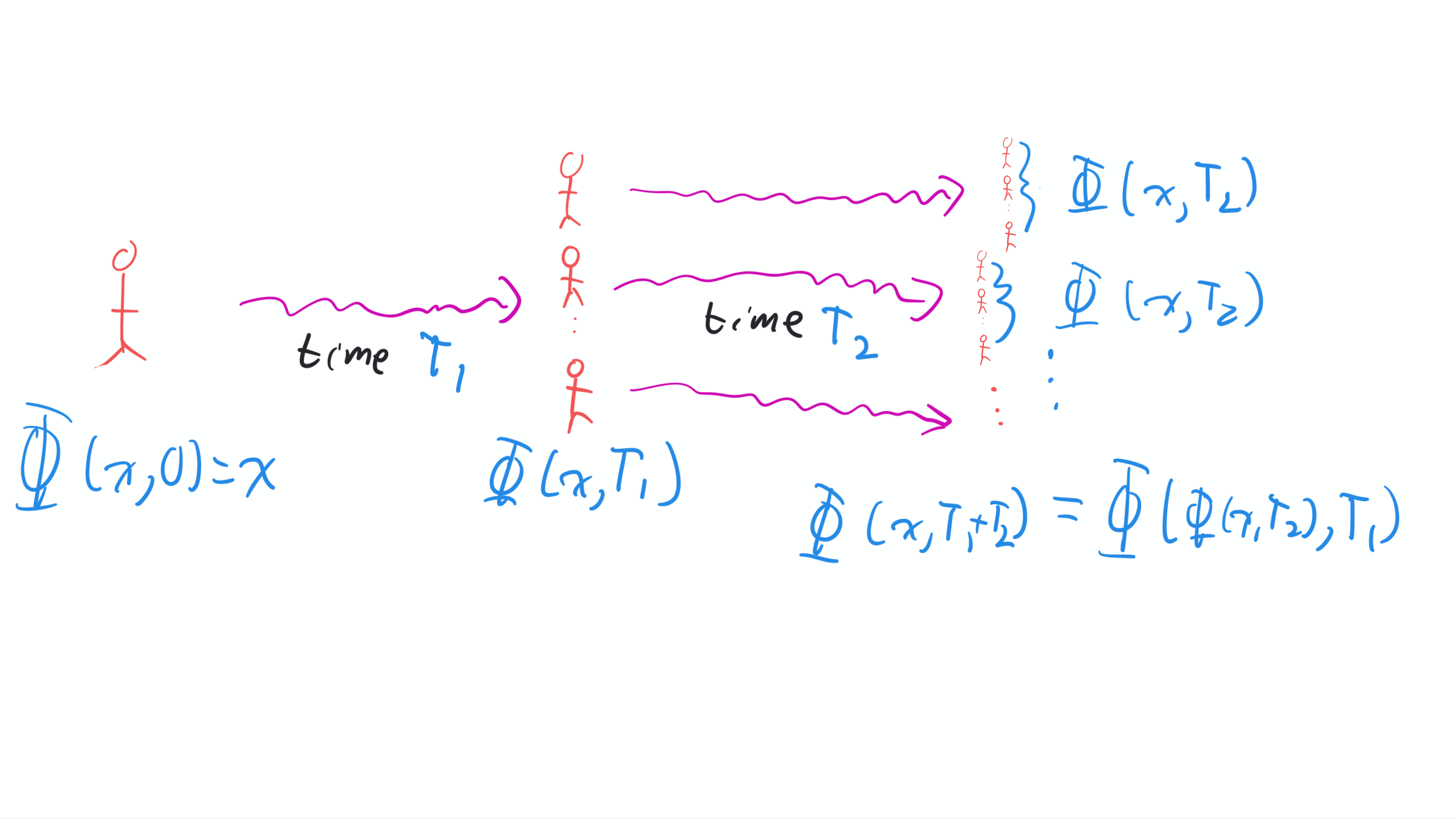
Fig. 3.2 Illustration of how \(\Phi(x,T_1+T_2)\) depends on \(\Phi(x,T_1)\) and \(\Phi(x,T_2)\).#
In our later derivations we will assume \(\Phi(x,t)\) is known. Then, in the Forward Kolmogorov Case we use \(T_1=t\) and \(T_2=\Delta t\) to find \(\Phi(x,t+\Delta t)\), which we then plug into the definition of the \(t\)-derivative to find \(\partial \Phi/\partial t\). The result is a differential equation for \(\Phi\). In the Backward Kolmogorov Case we use \(T_1=\Delta t\) and \(T_2=t\) to find a different differential equation for \(\Phi\) (which of course has the same solution \(\Phi(x,t)\), but offers up different information).
If you are comfortable with the lemma, then the derivation of the Kolmogorov equations will be short and relatively straightforward. If you are not comfortable with the lemma, then the derivation will be short and bewildering. So please spend some time coming to terms with this lemma before proceeding.
3.2.2. PGF at small times#
It will be important to know what the PGF of \(X(\Delta t)\) is when \(\Delta t \ll 1\).
We will ignore small terms in the derivation below. They could be kept and later shown to go to zero.
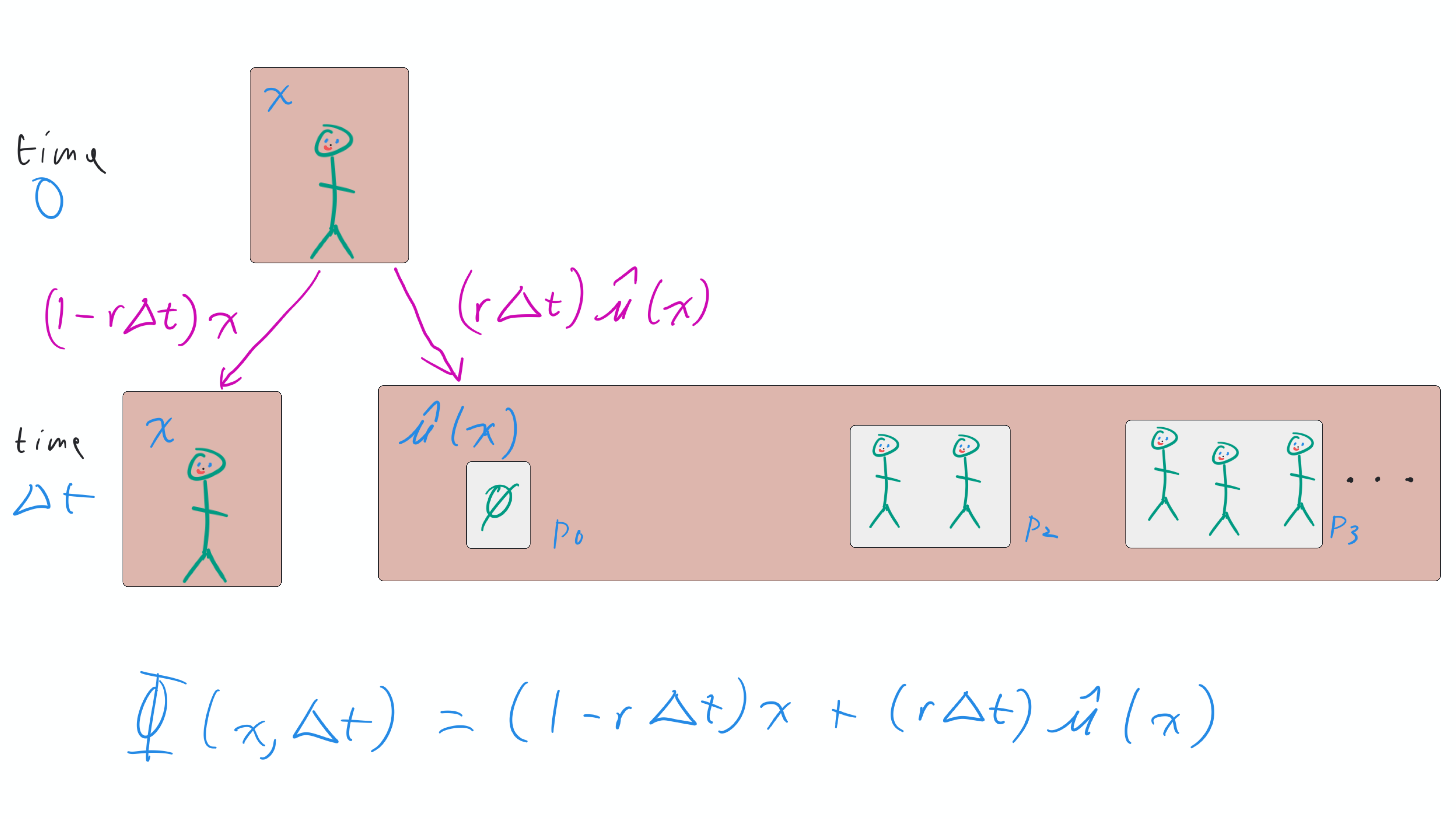
We begin with one individual at \(t=0\). The probability that the individual dies during the first \(\Delta t\) time units is (approximately) \(r \Delta t\). If so, the number of individuals replacing her has PGF \(\hat{\mu}(x)\). If not, then the resulting PGF is simply \(x\).
For sufficiently small \(\Delta t\), we can assume that at most one event occurs in the time interval. Then taking the appropriate convex combination of \(\hat{\mu}(x)\) and \(x\), we find
We turn this into a Lemma for future use, holding on to the small error terms that were neglected above:
Lemma 3.2 (PGF of \(X(t)\) at time \(\Delta t\))
If \(X(0)=1\), the PGF of the population size \(X(t)\) at time \(\Delta t \ll 1\) is
This is illustrated in Fig. 3.3
3.2.3. Mapping to the generation-based Galton-Watson process#
In defining \(\hat{\mu}(x)\), we assume that when an event happens an individual either dies (with probability \(p_0\)) or gives birth to \(k-1\) individuals (with probability \(p_k\), \(k>1\)), but we have treated it as if the individual dies and is replaced by \(k\) individuals. This assumption simplifies the calculations, but if we want to relate our results in the continuous time case to the generation-based case, we need to undo this assumption.
If we assume that the individual does not die in the birth events, then conditional on a birth event, the probability of having \(k\) offspring is \(q_k = p_{k+1}/(1-p_0)\). The corresponding PGF is:
The PGF for the number of birth events \(m\) comes from the geometric distribution, Example 1.9 (not counting the final event) is \(p_0/(1-(1-p_0)x)\).
Since the offspring distribution for the entire lifetime is a randomly stopped sum of \(m\) terms each with PGF \(\frac{ \hat{\mu}(x) - p_0}{(1-p_0)x}\), we have
3.2.4. Self-test#
Explain why we can assume \(p_1=0\) in the definition of \(\hat{\mu}(x)\). Hint: if there is one offspring and the parent is removed, what has changed?
If each birth event results in exactly one new individual (and the original individual remains present):
(a) Show that \(\hat{\mu}(x) = p_0 + (1-p_0)x^2\)
(b) Find \(\mu(x)\) for the generation-based model.
(c) Compare \(\mu(x)\) to the Geometric Distribution PGF Example 1.9 and explain why this process is equivalent to the coin flip description in Example 1.9.
It is relatively common to use the branching mechanism: \(\psi(x) = \sum_k r_k(x^k-x)\).
(a) Show that \(\psi(x) = r(\hat{\mu}(x) - x)\).
(b) Find the PGF \(\Phi(x,\Delta t)\) in terms of \(\psi\) rather than \(\hat{\mu}\).
(c) Explain why \(\psi(x)\) is not a PGF. (hint: what is \(\psi(1)\)?)
Consider Definition 3.4. We will try to understand why Definition 3.3 would follow. Assume the \(i\)th event occurs at time \(t_i\). Use the concept of superposition of Poisson processes to argue that
(a) The next event happens at a time \(t_{i+1}\) for which \(t_{i+1}-t_i\) is exponentially distributed with rate \(r X(t_i)\),
(b) The individual involved in the event can be randomly chosen from the population, and
(c) the probability that individual is replaced by \(k\) is \(p_k = r_k/r\).