1.8. Multiplication of Generating Functions

We’ll see that there are several uses for multiplication of two generating functions. First, we’ll look at the sequence of numbers that results from multiplying two generating functions together and then we’ll look at some applications.

Let’s assume we have two generating functions:

\[\begin{align*} f(x) &= f_0 + f_1 x + f_2 x^2 + \cdots\\ g(x) &= g_0 + g_1 x + g_2 x^2 + \cdots \end{align*}\]

We can represent multiplication of the sums through a table. Each column corresponds to a term of \(f(x)\) while each row corresponds to a term of \(g(x)\). The interior cells give the product of the corresponding terms of \(f(x)\) and \(g(x)\). The product \(f(x)g(x)\) will be the sum of all interior cells:

		\(\color{blue}{f_0}\)	\(\color{blue}{f_1x}\)	\(\color{blue}{f_2x^2}\)	\(\color{blue}{f_3x^3}\)	\(\color{blue}{f_4x^4}\)	\(\color{blue}{f_5x^5}\)	\(\cdots\)
\(\color{blue}{g_0}\)		\(f_0g_0\)	\(f_1g_0x\)	\(f_2g_0x^2\)	\(f_3g_0x^3\)	\(f_4g_0x^4\)	\(f_5g_0x^5\)	\(\cdots\)
\(\color{blue}{g_1x}\)		\(f_0g_1x\)	\(f_1g_1x^2\)	\(f_2g_1x^3\)	\(f_3g_1x^4\)	\(f_4g_1x^5\)	\(f_5g_1x^6\)	\(\cdots\)
\(\color{blue}{g_2x^2}\)		\(f_0g_2x^2\)	\(f_1g_2x^3\)	\(f_2g_2x^4\)	\(f_3g_2x^5\)	\(f_4g_2x^6\)	\(f_5g_2x^7\)	\(\cdots\)
\(\color{blue}{g_3x^3}\)		\(f_0g_3x^3\)	\(f_1g_3x^4\)	\(f_2g_3x^5\)	\(f_3g_3x^6\)	\(f_4g_3x^7\)	\(f_5g_3x^8\)	\(\cdots\)
\(\color{blue}{g_4x^4}\)		\(f_0g_4x^4\)	\(f_1g_4x^5\)	\(f_2g_4x^6\)	\(f_3g_4x^7\)	\(f_4g_4x^8\)	\(f_5g_4x^9\)	\(\cdots\)

We can illustrate this with an example:

Example 1.21 (Squaring \(\mu(x) = (x+x^2+x^3+x^4+x^5+x^6)/6\))

Consider squaring \(\mu(x) = \frac{x+x^2+x^3+x^4+x^5+x^6}{6}\). The product is illustrated in the figure below. Note that the terms that have the same exponent on \(x\) form a diagonal.

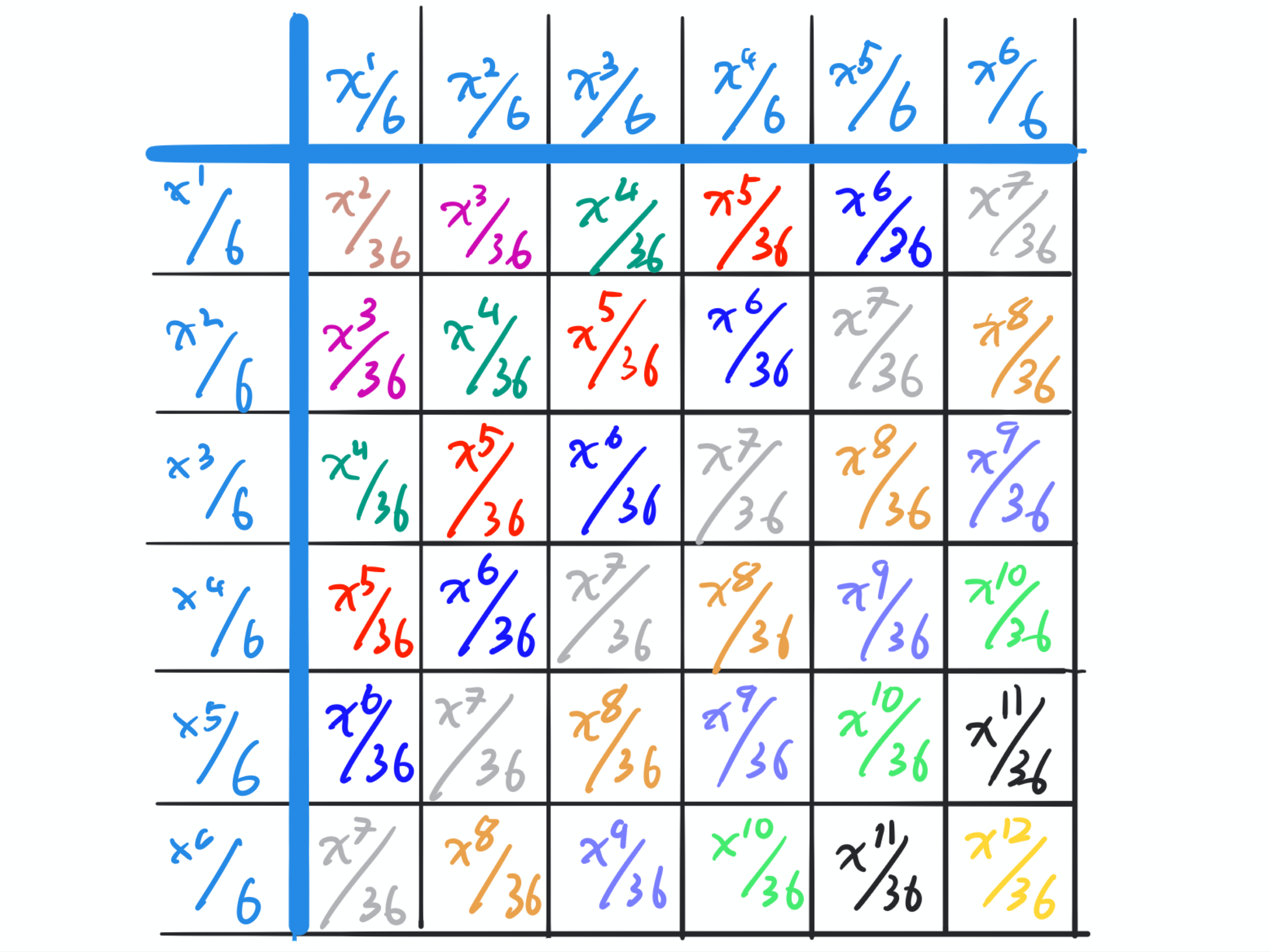
Fig. 1.6 The results of multiplying \(\mu(x) = (x+x^2+x^3+x^3+x^5+x^6)/6\) by itself following the table. The final result is the sum of the terms in each cell.

By looking at this table, we can see that each power of \(x\) shows up in a diagonal. The coefficient of \(x^n\) is equal to the sum of all products of the form \(f_k g_{n-k}\). That is,

\[ f(x) g(x) = \sum_{n=0}^\infty \left(x^n\sum_{k=0}^n f_kg_{n-k}\right) \]

We can express this using the \([x^n]h(x)\) notation (recall that this notation refers to the coefficient of \(x^n\) in the expansion of \(h(x)\)).

Theorem 1.2 (Convolution in series product)

Given two Generating Functions \(f(x) = f_0 + f_1 x + f_2 x^2 + \cdots\) and \(g(x) = g_0 + g_1 x + g_2 x^2 + \cdots\), then the coefficient of \(x^n\) in the product \(f(g)g(x)\) is given by

\[ [x^n](f(x)g(x)) = \sum_{k=0}^n f_k g_{n-k} \]

Writing it out in expanded form:

\[\begin{align*} f(x) g(x) =& f_0 g_0 + (f_1 g_0 + f_0 g_1) x + (f_2 g_0 + f_1 g_1 + f_0 g_2) x^2 \\&\quad+ \cdots + \left(\sum_{k=0}^n f_k g_{n-k}\right) x^n + \cdots \end{align*}\]

1.8.1. Partial sums of a sequence

An important special case occurs when \(f(x) = 1 + x + x^2 + \cdots = \frac{1}{1-x}\). Then

\[ f(x)g(x) = g_0 + (g_0+g_1) x + (g_0+g_1+g_2)x^2 + \cdots \]

This is a generating function whose coefficients are \(g_0\), \(g_0+g_1\), \(g_0+g_1+g_2\), \(\ldots\). These are the partial sums of the sequence \(g_0, g_1, \ldots\). So given a generating function \(g(x)\), we can construct the generating function of the partial sums by multiplying by \(\frac{1}{1-x}\).

Theorem 1.3 (Partial Sums)

Consider a sequence of numbers \(c_0, c_1, \ldots\) whose generating function is \(f(x)\). The partial sums

\[\begin{align*} s_0 &= c_0\\ s_1 &= c_0 + c_1\\ \end{align*}\]

and in general

\[ s_n = \sum_{i=0}^n c_i \]

have generating function \(\frac{f(x)}{1-x}\)

1.8.1.1. Cumulative probability

It follows quickly from Theorem 1.3 that given a probability distribution with probabilities \(p_0\), \(p_1\), \(\ldots\) whose probability generating function is \(\mu(x)\), the probability that a random number chosen from the distribution is less than or equal to \(n\) has generating function

\[ g(x) = \frac{\mu(x)}{1-x} = p_0 + (p_0+p_1)x + (p_0+p_1+p_2)x^2 + \cdots \]

Note that \(g(x)\) is an Ordinary Generating Function not a Probability Generating Function.

1.8.2. Multiplication of PGFs

The product of two PGFs will be particularly important to us.

Consider two PGFs, \(\mu_1(x) = \sum p_i x^i\) and \(\mu_2(x) = \sum q_j x^j\). Then \(\mu_1(x)\) is the PGF of the probability distribution for which (non-negative) integer \(i\) occurs with probability \(p_i\) and \(\mu_2(x)\) is the PGF for the distribution for which the probability of \(j\) is \(q_j\).

We will build a table giving the possible sums if we choose \(i\) from one distribution \(j\) from the other and the probability of choosing \(i\) and \(j\). It will resemble the table above. The cells at the edges have two entries: the probability of each integer from the corresponding distribution and the value of the integer. Each interior cell also has two entries, the probability that a particular pair \(i\) and \(j\) occurs and the sum \(i+j\).

		\(\color{blue}{p_0; \quad 0}\)	\(\color{blue}{p_1; \quad 1}\)	\(\color{blue}{p_2; \quad 2}\)	\(\color{blue}{p_3; \quad 3}\)	\(\color{blue}{p_4; \quad 4}\)	\(\color{blue}{p_5; \quad 5}\)	\(\cdots\)
\(\color{blue}{q_0; \quad 0}\)		\(p_0q_0; \quad 0\)	\(p_1q_0; \quad 1\)	\(p_2q_0; \quad 2\)	\(p_3q_0; \quad 3\)	\(p_4q_0; \quad 4\)	\(p_5q_0; \quad 5\)	\(\cdots\)
\(\color{blue}{q_1; \quad 1}\)		\(p_0q_1; \quad 1\)	\(p_1q_1; \quad 2\)	\(p_2q_1; \quad 3\)	\(p_3q_1; \quad 4\)	\(p_4q_1; \quad 5\)	\(p_5q_1; \quad 6\)	\(\cdots\)
\(\color{blue}{q_2; \quad 2}\)		\(p_0q_2; \quad 2\)	\(p_1q_2; \quad 3\)	\(p_2q_2; \quad 4\)	\(p_3q_2; \quad 5\)	\(p_4q_2; \quad 6\)	\(p_5q_2; \quad 7\)	\(\cdots\)
\(\color{blue}{q_3; \quad 3}\)		\(p_0q_3; \quad 3\)	\(p_1q_3; \quad 4\)	\(p_2q_3; \quad 5\)	\(p_3q_3; \quad 6\)	\(p_4q_3; \quad 7\)	\(p_5q_3; \quad 8\)	\(\cdots\)
\(\color{blue}{q_4; \quad 4}\)		\(p_0q_4; \quad 4\)	\(p_1q_4; \quad 5\)	\(p_2q_4; \quad 6\)	\(p_3q_4; \quad 7\)	\(p_4q_4; \quad 8\)	\(p_5q_4; \quad 9\)	\(\cdots\)

We compare the two tables, with the correspondence \(f(x)=\mu_1(x)\) so \(p_i = f_i\) and \(g(x)=\mu_2(x)\) so \(q_j = g_j\). In each cell of the second table, the product \(p_iq_j\) matches the coefficient of the equivalent cell of the first table. The sum \(i+j\) matches the exponent of \(x\) of the equivalent cell the first table. This suggests that adding random numbers and multiplying PGFs are closely related processes.

More generally, given two PGFs

\[\begin{align*} \mu_1(x) &= \sum_n p_n x^n\\ \mu_2(x) &= \sum_n q_n x^n \end{align*}\]

If we choose \(K\) from the distribution with PGF \(\mu_1(x)\) and \(M\) from the distribution with PGF \(\mu_2(x)\), then the sum \(K+M\) is a random non-negative integer. The probability of a particular pair \(K=k\), \(M=m\) is \(p_kq_m\). The probability of a given sum \(n\) is found by adding up the probabilities \(p_kq_m\) for which \(k+m=n\), that is \(\sum_{k=0}^\infty p_k q_{n-k}\) .

Theorem 1.4 (PGF of random sum)

Given the PGFs

\[\begin{align*} \mu_1(x) &= \sum_n p_n x^n\\ \mu_2(x) &= \sum_n q_n x^n \end{align*}\]

If we choose \(K\) from the distribution with PGF \(\mu_1(x)\) and \(M\) from the distribution with PGF \(\mu_2(x)\), then the probability \(\mathbb{P}[K+M=n]\) is

\[ \mathbb{P}[K+M=n] = \sum_{k=0}^n p_k q_{n-k} \]

and the PGF of the sum is

\[ \psi(x) = \mu_1(x)\mu_2(x) \]

Proof. The probability of a sum \(n\) is \(\sum_{k=0}^n p_k q_{n-k}\). So the PGF of the sum is

\[ \sum_{n=0}^\infty \left(\sum_{k=0}^n p_n q_{n-k}\right) x^n \]

However, this is also \(\psi(x)=\mu_1(x)\mu_2(x)\) from Theorem 1.2. Thus the PGF of the sum \(K+M\) is equal to \(\psi(x)=\mu_1(x)\mu_2(x)\).

This is a very important result. By repeatedly applying this argument, it generalizes to products of multiple PGFs. We enshrine this in a corollary:

Corollary 1.1 (Product of PGFs)

Given \(k\) PGFs \(\mu_1(x), \mu_2(x), \ldots, \mu_k(x)\), the product

\[ \psi(x) = \prod_{i=1}^k \mu_i(x) \]

is also a PGF and it corresponds to the probability distribution of the sum \(n_1 + n_2 + \cdots + n_k\) where each \(n_i\) comes from the distribution whose PGF is \(\mu_i(x)\).

Proof. The proof of this follows from induction and the fact that \(\psi(x)=\mu_1(x)\mu_2(x)\) is the PGF of the sum of the two random numbers.

1.8.2.1. Powers of PGFs

A further corollary of Corollary 1.1 is found by assuming \(\mu_1(x) = \mu_2(x) = \cdots = \mu_k(x) = \mu(x)\).

Corollary 1.2 (PGF of sum of repeated draws)

Given a PGF \(\mu(x)\), if we perform \(k\) draws from its distribution, the PGF for the sum of all \(k\) draws is \(\mu(x)^k\).

This explains the observation made in Remark 1.4 that the PGF for the number of heads out of \(n\) flips of a weighted coin \([(1-p_H) + p_Hx]^n\) is the \(n\)-th power of the PGF for a single flip.

Example 1.22 (Sicherman Dice)

Consider two standard dice, with the PGF \(\psi(x) = (x + x^2 + x^3 + \cdots +x^6)/6\). We are interested in the sums we get when we roll them:

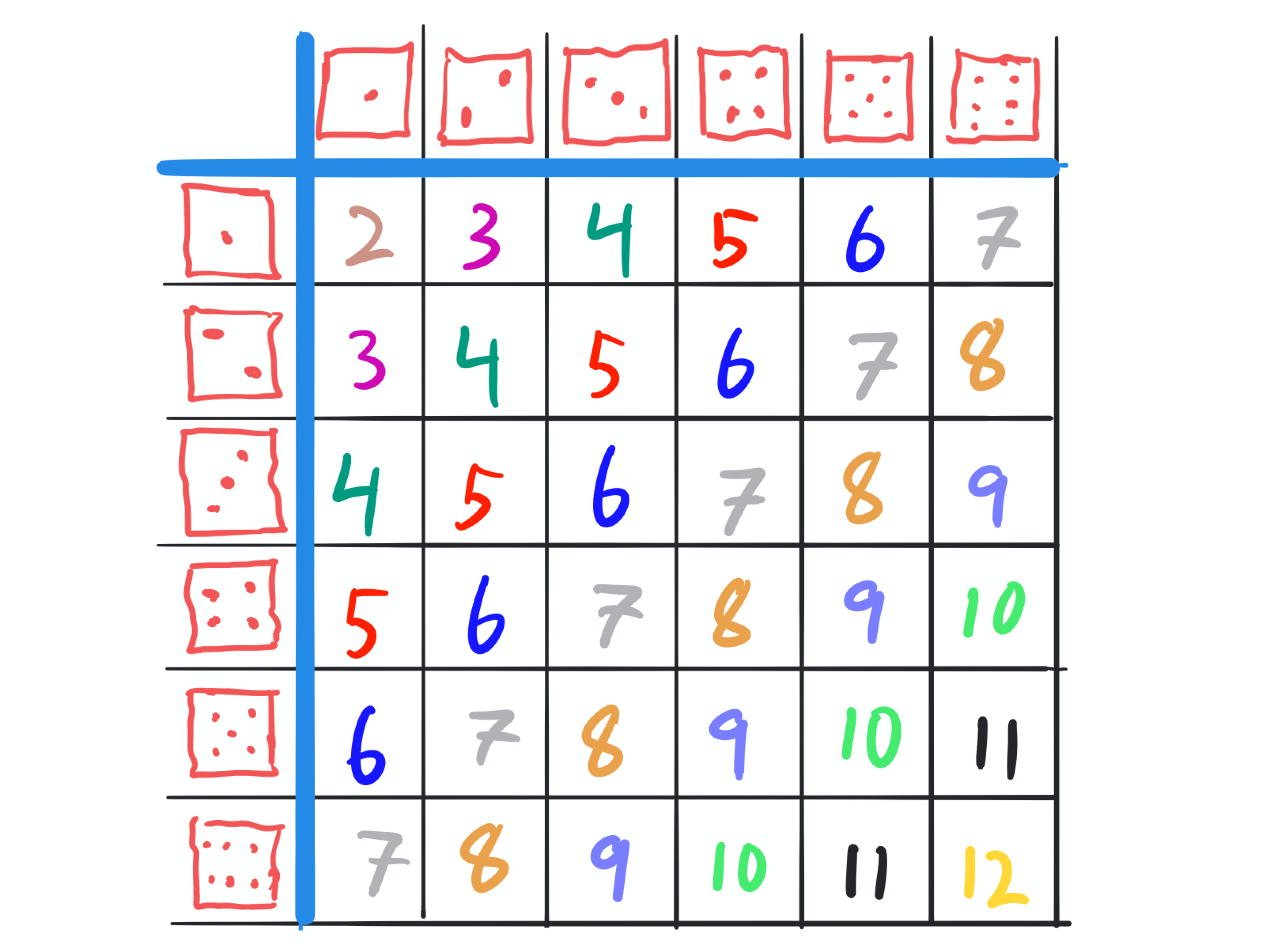
Fig. 1.7 The sums from a standard pair of dice. Each grid cell has probability \(1/36\).

When we roll the two dice, the PGF for their sum is \([\psi(x)]^2\). An interesting challenge is to determine whether it is possible to find another pair of fair 6-sided dice that give the same sums with the same probabilities as the standard dice.

If we set aside PGFs for a moment, it is relatively straightforward to see that if we require that the two dice be identical to one another then they must be a standard pair. The argument starts by showing that if the minimum combined roll is 2, with probability \(1/36\), and the dice are identical, they must each have a \(1\). Then looking at the next value of \(3\) with probability \(2/36\), we can conclude they each have a \(2\). Extending this process will finish the proof.

However, if we allow the two dice to be different it is possible to find other pairs. The easiest way to do this is simply to add a constant to everything on one die and subtract that same constant from everything on the other die. This isn’t very exciting.

A more interesting challenge is the following:

Is there a pair of 6-sided dice with positive integer values which gives the same sums with the same probabilities as a standard pair of dice? If so, is it unique?

We’ll translate this question into PGFs: Are there two PGFs that can be written

\[\begin{align*} \mu_1(x) &= \frac{1}{6} \left[ x^{i_1} + x^{i_2} + \cdots + x^{i_6}\right]\\ \mu_2(x) &= \frac{1}{6} \left[ x^{j_1} + x^{j_2} + \cdots + x^{j_6}\right] \end{align*}\]

Such that \([\psi(x)]^2 = \mu_1(x)\mu_2(x)\)?

Before continuing, please ensure that you understand why this question is equivalent to the original dice question.

We begin by fully factoring \([\psi(x)]^2\):

\[\begin{align*} [\psi(x)]^2 &= \frac{1}{36} (x+x^2+x^3+x^4+x^5+x^6)^2\\ &= \frac{1}{36} [x(1+x+x^2+x^3+x^4+x^5)]^2\\ &= \frac{1}{36} [x(1+x+x^2)(1+x^3)]^2\\ &= \frac{1}{36} [x(1+x+x^2)(1+x)(1-x+x^2)]^2\\ &= \frac{1}{2^2 3^2} x^2(1+x+x^2)^2(1+x)^2(1-x+x^2)^2 \end{align*}\]

This is fully factored over polynomials with real coefficients. This is the polynomial equivalent of a prime factorization of \([\psi(x)]^2 = \mu_1(x)\mu_2(x)\). These factors must be shared between \(\mu_1(x)\) and \(\mu_2(x)\). If each the factors are all shared equally then \(\mu_1(x)=\mu_2(x)=\psi(x)\) and we recover the standard pair. To find another pair, we must distribute some of the factors unequally, and we must also ensure that the final polynomials that result are PGFs of the form identified above.

We now identify two constraints on the PGFs:

• \(\mu_1(0)=\mu_2(0)=0\) because we have insisted on positive integer values for the dice. Thus when we plug \(0\) into \(\mu_1(x)\) and \(\mu_2(x)\), we must get the probability of \(0\) which is zero.

• \(\mu_1(1)=\mu_2(1)=1\) because for any PGF, its value at \(x=1\) is \(1\).

Notice that at \(x=0\), the only factor that gives \(0\) is \(x\), while at \(x=1\), the factor \(1+x+x^2\) is \(3\) and \(1+x\) is \(2\), while \((1-x+x^2)\) is \(1\). From these observations, we conclude that the factors \(x\), \(1+x\), and \(1+x+x^2\) must be shared equally between the dice, but we do not have any condition on \((1-x+x^2)\). Thus:

\[\begin{align*} \mu_1(x) &= \frac{1}{6} x(1+x+x^2)(1+x) (1-x+x^2)^{2-a}\\ \mu_2(x) &= \frac{1}{6} x(1+x+x^2)(1+x) (1-x+x^2)^a\\ \end{align*}\]

where \(a\) could be \(0\), \(1\), or \(2\). If \(a=1\), we recover the standard pair of dice. If \(a=0\):

\[\begin{align*} \mu_1(x) &= \frac{1}{6} x(1+x+x^2)(1+x) (1-x+x^2)^{2}\\ \mu_2(x) &= \frac{1}{6} x(1+x+x^2)(1+x) \\ \end{align*}\]

While \(a=2\) simply interchanges \(\mu_1(x)\) and \(\mu_2(x)\).

So we have a candidate pair, but we have not yet shown that these are definitely PGFs of the desired form. We must expand the products out and see that they look like. We get

\[\begin{align*} \mu_1(x) &= \frac{x+ x^3 + x^4 +x^5 + x^6 + x^8}{6}\\ \mu_2(x) &= \frac{x +2x^2 + 2x^3 + x^4}{6} = \frac{x + x^2 + x^2 + x^3 + x^3 + x^4}{6} \end{align*}\]

These are PGFs for a pair of dice numbered \(1,3,4,5,6,8\) and \(1,2,2,3,3,4\). This pair will yield the same sums with the same probabilities as a standard pair of dice. This pair of dice is known as Sicherman Dice. Our approach further shows that there can be no other pair of \(6\)-sided dice with positive integer values that give the same sums.

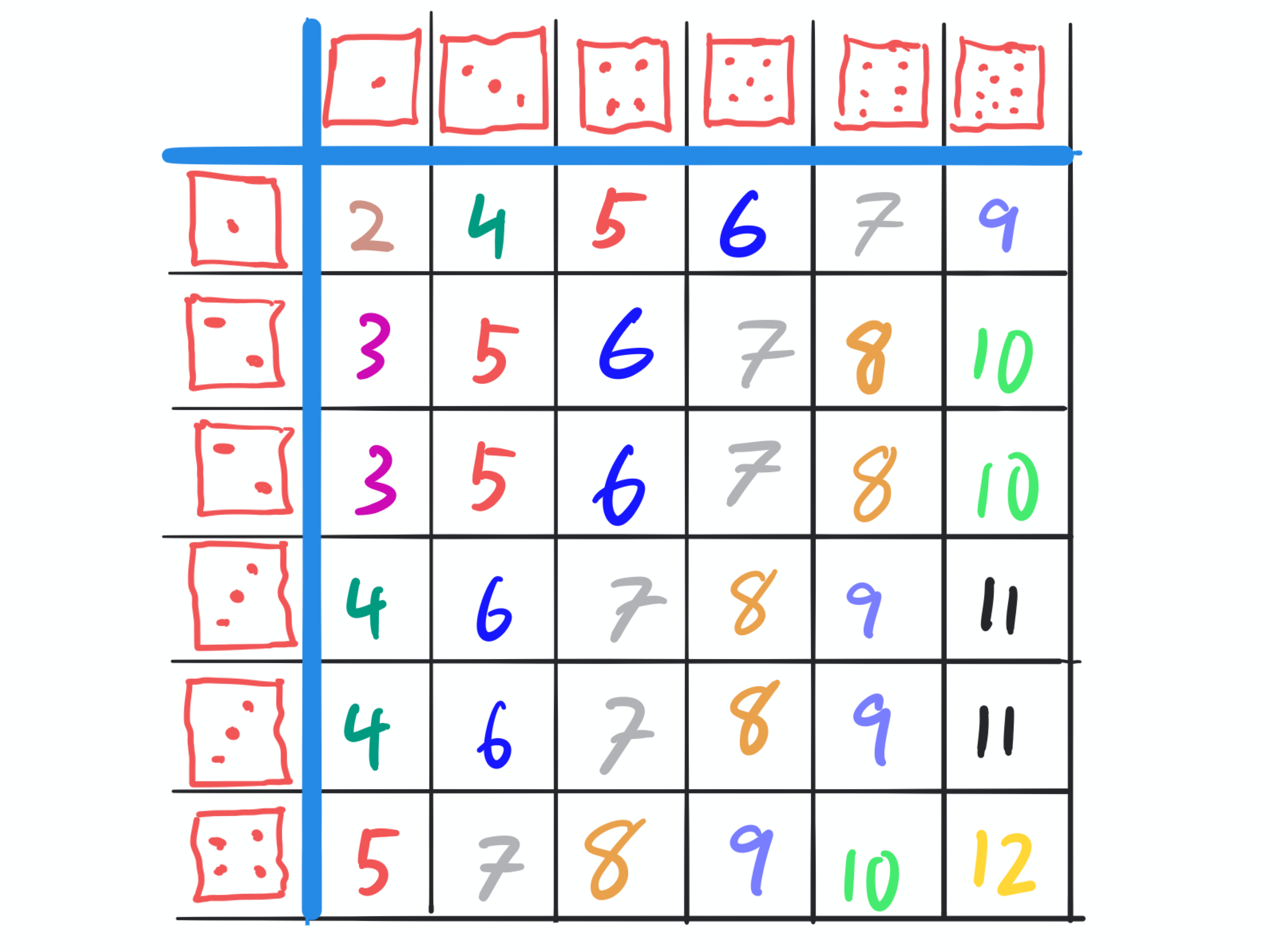
Fig. 1.8 The results of rolling a pair of Sicherman Dice. The same sums occur with the same probabilities as with a standard pair.

1.8.3. Self-test

I added a question about stop lights after this went “live”. I have put it at the end, but I should re-order the questions in the future. I’ve also added a question to find the expected value of the sum of \(k\) random variables.

1. We will verify the identity \(F_{n+2}-1 = \sum_{i=0}^n F_i\) for partial sums of the Fibonnaci sequence. Let \(f(x) = F_0 + F_1 x + \cdots\) which we have shown equals \(x/(1-x-x^2)\).

   1. Let

      \[g(x) = \frac{f(x)}{1-x} \]

      Which we have noted gives the generating function for partial sums of the coefficients of \(f\). By writing \(f(x)\) in the form \(\sum_i F_i x^i\) and \(1/(1-x)\) in the form \(\sum_i x^i\) do term-by-term multiplication to find all terms of \(g(x)\) up to \(x^3\), to verify that \(g(x)\) our claim, at least up to \(x^3\) (and it should be clear to you why this continues for higher powers).

   2. Define

      \[h(x) = \sum_{n=1}^\infty F_{n+2}x^n \]

      Consider the function \(k(x) = h(x) - \frac{1}{1-x}\). How is \(k(x)\) related to the sequence \(F_{n+2}-1\)?

   3. Look at the terms of \(h(x)x^2\) and \(f(x)\). Use this to write \(h(x)x^2\) as \(f(x)\) plus a low-degree polynomial. Use Algebra to convert this into an equation for \(h(x)\) in terms of \(f(x)\) and a low degree polynomial.

   4. Write \(k(x)\) in terms of \(f(x)\) and compare it with \(g(x)\). What can you conclude?

2. This problem gives a preview of the material in the next section. Let \(\mu(x) = (x+x^2+x^3+x^4+x^5+x^6)/6\), the PGF of a standard die.

   1. What is \(A_k(x) = [\mu(x)]^k\) the PGF for, in terms of the sum of some dice rolls?

   2. Consider the following process: roll a standard die to get a number \(k\). Then roll \(k\) dice and sum their values to get \(n\). Let \(\psi(x)\) be the PGF for the resulting distribution of \(n\). Using the previous section’s results for linear combinations of PGFs, write \(\psi(x)\) in terms of \(A_k(x)\), \(k=1, \ldots, 6\).

   3. Show that \(\psi(x) = \mu(\mu(x))\).

3. Consider two “standard” \(4\)-sided (tetrahedral) dice numbered \(1,2,3,4\). Find another pair of \(4\)-sided dice with positive integer values, analagous to the Sicherman Dice which give the same sums with the same probabilities as the standard pair.

4. Consider two “standard” \(4\)-sided (tetrahedral) dice numbered \(1,2,3,4\).

   1. Find an octahedral (8-sided) die and a coin, both with positive integer values on each side such that flipping the coin and rolling the die give the same sums with the same probabilities as a standard pair of tetrahedral dice.

   2. Is this die-coin pair unique? If not, find another example.

5. Consider the Ordinary Generating Function \(f(x)=\frac{1}{1-x}=1+x+x^2+\cdots\).

   1. Use its multiplication properties to find a compact expression for the OGF \(0 + x + 2x^2 + 3x^3 + \cdots\) in terms of \(1/(1-x)\).

   2. Use differentiation of \(f(x)\) to find the find the same OGF.

6. Explain why Remark 1.5 is true.

7. A stoplight allows a random number of vehicles \(V\) through each cycle. The PGF is \(\mu(x)\). What is the PGF \(\psi_k(x)\) of the number it would allow through in \(k\) cycles?