8.1. Assignment 1

This will be due Friday 23 Jan, 11:59PM. I’ll set up a submission portal on Moodle.

Please do not use AI to assist with these. I plan to do some “auditing” of solutions to make sure you can reproduce the answers you submit. I will update these instructions with guidance about a prompt that you can use with AI systems to get help on these.

If you get help or give help to anyone else, please find a similar problem to discuss. Do not directly work on a problem in the question.

These problems are not ordered by difficulty. They are ordered roughly with where the corresponding material appears in the text. I have a reputation for setting long assignments (I get excited by what each problem can reveal to students). I will have consultation hours next week (and I will make sure that you can reach me on zoom if you are remote). As I see where people struggle, I may add hints to these questions.

8.1.1. Instructions for AI use:

Never trust anything that can think for itself if you can’t see where it keeps its brain.

— Arthur Weasley, Harry Potter and the Chamber of Secrets

AI can be an amazing learning tool. It is also amazingly effective at preventing learning. There is a lot of benefit in looking at a problem on your own, thinking about how to solve it, and even running into dead-ends when you attempt the wrong method.

Here are the guidelines for use of AI on this problem set:

1. Before turning to AI for assistance on a question, think about the question yourself. Identify what the question is asking and make some attempt to solve it on your own.

2. If you use an AI, you must save the “conversation” you have.

3. You must start the conversation with the prompt below, and you cannot encourage the AI to violate the prompt.

4. You must complete the “Learning Reflection” below for each question on which you used AI.

8.1.1.1. AI Prompt

I am working on a problem that I must solve on my own. Please do not give me the full solution. Instead:

• Find a similar problem to solve.

• Ask me questions to check whether I understand each step.

• Only reveal the next step after I attempt it.

• If I make a mistake, respond with hints instead of the correct answer.

My goal is to understand and be able to solve similar problems without AI.

8.1.1.2. Learning Reflection

• What did I already know about this problem before asking AI?

• What did I learn?

• What detail or technique was the most important for completing this problem?

(3-6 sentences maximum)

8.1.2. Problem set

Any edits since the assignment was released are in bold

1. Let \(X\) be a discrete random variable with distribution

   \[ \mathbb{P}[X=0] = 0.2, \quad \mathbb{P}[X=1] = 0.5, \quad \mathbb{P}[X=2] = 0.3. \]

   (a) Find the probability generating function \(\psi(x)\) of this distribution.

   Solution (a)

   \[\begin{align*} \psi(x) &= \sum_k \mathbb{P}[X=k] x^k\\ &= 0.2 + 0.5x + 0.3x^2 \end{align*}\]

   (b) Use the probability generating function to compute the expected value \(\mathbb{E}[X]\).

   Solution (b)

   \[ \mathbb{E}[x] = \psi'(1) = 0.5 + 0.6\cdot 1 = 1.1 \]

2. Suppose a generating function is defined as

   \[ f(x) = \sum_{n=0}^{\infty} c_n x^n, \]

   and you are given that

   \[ f(x) = e^x = \sum_{n=0}^{\infty} \frac{x^n}{n!}. \]

   (a) According to the generating-function paradigm, what sequence \((c_n)\) does the function \(f(x)\) represent?

   Solution (a)

   \[ f(x) = \sum c_n x^n \]

   So

   \[ c_n = \frac{1}{n!} \]

   (b) Explain how the generating-function paradigm interprets \(f(x)\) as a compact way of encoding this sequence. In your explanation, describe how the coefficients \(c_n\) can be recovered from the function using derivatives evaluated at \(x = 0\).

   Solution (b)

   The function \(f(x)\) encodes the sequence because we an recover the coefficients \(c_n\) through repeated derivatives: \(c_n = \left. \frac{1}{n!} \frac{d^n}{dx^n} e^x \right|_{x=0}\).

3. Let \(X\) be a discrete random variable with values \(\{0,1,2,\ldots\}\) and

   \[ \mathbb{P}[X = k] = C \left(\frac{1}{2}\right)^k \quad \text{for } k = 0,1,2,\ldots \]

   where \(C\) is a normalizing constant.

   (a) Determine the value of \(C\).

   Solution (a)

   We need the sum of the probabilities to be \(1\), so

   \[\begin{align*} C &= \left( \sum_k \left(\frac{1}{2}\right)^k\right)^{-1}\\ &= \left( \frac{1}{1-1/2}\right)^{-1}\\ &= 2^{-1}\\ &= 1/2 \end{align*}\]

   (b) Find the probability generating function \(\mu(x)\) in closed form.

   Solution (b)

   \[\begin{align*} \mu(x) &= \sum_k \mathbb{P}[X=k]x^k\\ &= \sum_k \frac{1}{2} \left(\frac{1}{2}\right)^kx^k\\ &= \frac{1}{2}\frac{1}{1-x/2}\\ &= \frac{1}{2-x} \end{align*}\]

   (c) Use \(\mu(x)\) and \(x \partial_x\) to find \(\sum_k k^2/2^k\).

   Solution (c)

   Applying \(x \partial_x\) to a generating function \(\sum_k c_kx^k\) yields \(\sum_k k c_k x^k\). Applying it twice yields \(\sum_k k^2 c_k x^k\). So:

   \[\begin{align*} \sum_k C\frac{k^2}{2^k} x^k&=(x\partial_x)^2 \mu(x)\\ &= x\partial_x \left(x \partial_x (2-x)^{-1}\right) \\ &= x \partial_x \left(x (-1)(2-x)^{-2}(-1)\right)\\ &= x \partial_x\left( x(2-x)^{-2}\right)\\ &= x\left( (2-x)^{-2} + x(-2)(2-x)^{-3}(-1)\right)\\ &= \frac{x}{(2-x)^2} + \frac{2x^2}{(2-x)^3} \end{align*}\]

   So evaluating at \(x=1\) gives \(C\sum k^2/2^k = 1/1^2 + 2/1^3 = 3\). Since \(C=1/2\), we conclude that

   \[ \sum_k k^2/2^k = 6 \]

4. In high school I came across a method that seemed to find all of the numbers that are both triangular numbers \((m)(m+1)/2\) and square numbers \(n^2\) (I couldn’t prove it at the time).

   Consider the sequence \(a_n\) defined by \(a_0=1\), \(a_1=2\) and \(a_{n+2} = a_n + 2a_{n+1}\) and the sequence \(b_n\) defined by \(b_0=1\), \(b_1 = 3\) and \(b_{n+2} = b_n + 2b_{n+1}\). Then \((a_nb_n)^2\) is both triangular and square.

   I’ve since learned that this property of the sequence is known, but it’s still an interesting result. We can use OGFs to prove that these are both triangular and square (though it doesn’t prove that every triangular and square number is in the sequence). Some of these steps follow our derivation of the formula for the Fibonacci numbers.

   (a) For \(n=0, 1, 2\) (only these three values) use direct calculation to verify \(b_n^2 + (-1)^n = 2a_n^2\). Thus it follows that \((a_nb_n)^2 = b_n^2(b_n^2\pm 1)/2\) is both square and triangular. Now we want to show this for the general case, and be able to quickly find the \(n\)-th such number.

   note to self — to update this question, ask them to verify that \((a_nb_n)^2\) is a triangular number by finding \(m(m+1)/2 = a_n^2b_n^2\)

   Solution (a)

   \(n=0\):

   We have \(a_0=1\) and \(b_0=1\). For the LHS

   \[\begin{align*} b_0^2 +(-1)^0 &= 1+1\\ &=2 \end{align*}\]

   and for the RHS:

   \[ 2a_0^2 = 2 \]

   So these are equal.

   \(N=1\):

   We have \(a_1=2\) and \(b_1=3\). For the LHS

   \[\begin{align*} b_0^2 +(-1)^1 &= 9-1\\ &=8 \end{align*}\]

   and for the RHS:

   \[\begin{align*} 2a_1^2 &= 2\cdot 4\\ &= 8 \end{align*}\]

   So these are equal.

   \(N=2\):

   We have \(a_1=5\) and \(b_1=7\). For the LHS

   \[\begin{align*} b_0^2 +(-1)^2 &= 49+1\\ &=50 \end{align*}\]

   and for the RHS:

   \[\begin{align*} 2a_1^2 &= 2\cdot 25\\ &= 50 \end{align*}\]

   So these are equal.

   The numbers \(b_n^2a_n^2\) are \(1=1^2=1(2)/2\), \(36=6^2=8(9)/2\), and \(1225 = 35^2=49(50)/2\).

   As an interesting aside, the best rational approximations to \(\sqrt{2}\) are: \(1/1, 3/2, 7/5, 17/12, 41/29, \ldots, b_n/a_n, \ldots\). In this context what it means to say \(b_n/a_n\) is the “best” is that any rational approximation to \(\sqrt{2}\) that is closer than \(b_n/a_n\) must have a denominator that is larger than \(a_n\). So for example \(7/5\) is closer to \(\sqrt{2}\) than any other rational number with a denominator less than \(11\) and \(17/12\) is closer to \(\sqrt{2}\) than any rational number with a denominator less than \(29\).

   (b) Derive the OGFs \(f(x)\) and \(g(x)\) for both \(a_n\) and \(b_n\). Please disregard my prior advice about what this function should look like. I misplaced my calculations when I wrote the question. Ultimately, you should end up with something that gets a simple expression for \(a_n\) in (d) that somewhat resembles the expression stated for \(b_n\).

   Solution (b)

   Both have the same recurrence relationship, but with a different value of the second term. We will start with \(f(x)\), but in full generality, not using the values of \(a_0\) or \(a_1\). Thus the result will apply to \(g(x)\) as well.

   \[\begin{align*} f(x) &= a_0 + a_1 x + \sum_{n=2}^\infty a_n x^n\\ &= a_0 + a_1 x + \sum_{n=2}^\infty (a_{n-2} + 2a_{n-1})x^n\\ &= a_0 + a_1 x + \sum_{n=2}^\infty a_{n-2}x^n + \sum_{n=2}^\infty + 2a_{n-1}x^n\\ &= a_0 + a_1 x + \sum_{m=0}^\infty a_{m}x^{m+2} + \sum_{m=1}^\infty + 2a_{m}x^{m+1} \end{align*}\]

   where we are reindexing by setting \(m=n-2\) and then \(m=n-1\) in the two sums. Continuing:

   \[\begin{align*} f(x) &= a_0 + a_1 x + x^2 \sum_{m=0}^\infty a_mx^m + 2x \sum_{m=1}^\infty a_mx^m\\ &= a_0 + a_1 x + x^2 f(x) + 2x \left( -a_0 + a_0 + \sum_{m=1}^\infty a_mx^m\right)\\ &= a_0 + a_1 x + x^2 f(x) + 2x \left( -a_0 +\sum_{m=0}^\infty a_mx^m\right)\\ &= a_0 + a_1 x + x^2 f(x) + 2x\left( f(x) - a_0\right)\\ &= a_0 + a_1 x + x^2 f(x) + 2xf(x) - 2xa_0\\ \Rightarrow (1-x^2-2x)f(x) &= a_0 + x(a_1 - 2a_0)\\ \Rightarrow f(x) &= \frac{a_0 + x(a_1-2a_0)}{1-2x-x^2} \end{align*}\]

   Applying this to \(f(x)\) with \(a_0=1\) and \(a_1=2\) yields

   \[ f(x) = \frac{1}{1-2x-x^2} \]

   and applying it to \(g(x)\) with \(b_0=1\) and \(b_1=3\) yields

   \[ g(x) = \frac{1 + x}{1-2x-x^2} \]

   (c) Let \(Q= 1+\sqrt{2}\) and \(R = 1-\sqrt{2}\). Your denominators for the OGFs should equal \((1-Qx)(1-Rx)\). Write \(f(x) = A/(1-Qx) + B/(1-Rx)\). Find \(A\) and \(B\) in terms of \(Q\) and \(R\).

   Solution (c)

   Using \(Q=1+\sqrt{2}\) and \(R=1-\sqrt{2}\) the denominator factors as \((1-Qx)(1-Rx)\). For \(f(x)\), we have

   \[\begin{align*} \frac{1}{1-2x-x^2} &= \frac{A}{1-Qx} + \frac{B}{1-Rx}\\ \Rightarrow 1 &= A(1-Rx) + B(1-Qx) \end{align*}\]

   There are multiple options from here. The simplest is to set \(x=1/R\) and \(x=1/Q\):

   \(x=1/R\):

   \[\begin{align*} 1 &= A(0) + B(1-Q/R)\\ &= B\frac{R-Q}{R}\\ \Rightarrow B &= \frac{R}{R-Q} \end{align*}\]

   \(x=1/Q\):

   \[\begin{align*} 1 &= A(1-R/Q) + B(0)\\ &= A\frac{Q-R}{Q}\\ \Rightarrow A &= \frac{Q}{Q-R}\\ &= - \frac{Q}{R-Q} \end{align*}\]

   The last step isn’t needed, but it makes the denominators the same, so it’s likely to simplify algebra later.

   (d) Use this to write \(a_n\) in terms of \(Q\) and \(R\). Similar steps show that \(b_n = (Q^{n+1} + R^{n+1})/2\).

   Solution (d)

   We have

   \[\begin{align*} f(x) &= \frac{A}{1-Qx} + \frac{B}{1-Rx}\\ &= \frac{1}{R-Q} \left (\frac{-Q}{1-Qx} + \frac{R}{1-Rx}\right)\\ &= \frac{1}{R-Q} \left ( -Q \sum_{n=0}^\infty Q^nx^n +R \sum_{n=0}^\infty R^nx^n\right)\\ &= \frac{1}{R-Q} \sum (R^{n+1}-Q^{n+1})x^n \end{align*}\]

   So the coefficient of \(x^n\) is \(a_n=\frac{R^{n+1}-Q^{n+1}}{R-Q}\)

   (e) Write \(b_n^2\) in terms of \(Q\) and \(R\), simplifying any \(QR\) term using \(QR=-1\).

   Solution (e)

   We are given that \(b_n= (Q^{n+1}+R^{n+1})/2\). So \(b_n^2 = (Q^{2n+2} + 2(QR)^{n+1} + R^{2n+2})/4\). Since \(QR=-1\) we can simplify the middle term so

   \[ b_n^2 = \frac{Q^{2n+2} + R^{2n+2} + 2(-1)^{n+1}}{4} = \frac{Q^{2n+2}+R^{2n+2}}{4} + \frac{(-1)^{n+1}}{2} \]

   (f) Similarly simplify \(2a_n^2\) in terms of \(Q\) and \(R\), and show that \(2a_n^2 = b_n^2 + (-1)^n\).

   Solution (f)

   We get

   \[\begin{align*} 2 a_n^2 &= 2\left(\frac{R^{n+1}-Q^{n+1}}{R-Q}\right)^2\\ &= 2\frac{ R^{2n+2} - 2(QR)^{n+1} + Q^{2n+2}}{(R-Q)^2} \\ &= \frac{2}{(-2\sqrt{2})^2} \left(Q^{2n+2} -2(-1)^{n+1} + R^{2n+2}\right)\\ &= \frac{Q^{2n+2}+R^{2n+2}}{4} - \frac{(-1)^{n+1}}{2} \end{align*}\]

   where \(R-Q = -2\sqrt{2}\) was used in the third line. Now adding zero in a disguised form:

   \[\begin{align*} 2a_n^2 &= \frac{Q^{2n+2}+R^{2n+2}}{4} + \left(\frac{(-1)^{n+1}}{2}-\frac{(-1)^{n+1}}{2}\right) - \frac{(-1)^{n+1}}{2}\\ &= \left(\frac{Q^{2n+2}+R^{2n+2}}{4} + \frac{(-1)^{n+1}}{2}\right)+ \left(-\frac{(-1)^{n+1}}{2} - \frac{(-1)^{n+1}}{2}\right)\\ &= b_n^2 - (-1)^{n+1}\\ &= b_n^2 + (-1)^n \end{align*}\]

   (g) Thus explain why \(b_n^2 a_n^2\) is a triangular number (it is clearly square).

   Solution (g)

   Since \(a_n^2 = \frac{b_n^2+(-1)^n}{2}\), we have

   \[\begin{align*} a_n^2 b_n^2 &= \frac{(b_n^2)(b_n^2 + (-1)^n)}{2}\\ &= \begin{cases} \frac{b_n^2(b_n^2+ 1)}{2} & n\text{ even}\\ \frac{(b_n^2 - 1)b_n^2}{2} & n\text{ odd} \end{cases} \end{align*}\]

   So this is either the \(b_n^2\)-th or \(b_n^2-1\)-th triangular number.

5. (a) Show how the variance of a distribution can be written using derivatives of a PGF evaluated at \(1\).

   Solution (a)

   The variance is \(\mathbb{E}[X^2] - \mathbb{E}[X]^2\). For the PGF \(\mu(x)\), we have

   \[\begin{align*} \mu'(1) &= \sum_k k p_k 1^{k-1}\\ &= \mathbb{E}[X] \end{align*}\]

   and

   \[\begin{align*} \mu''(1) &= \sum_k k(k-1) p_k 1^{k-2}\\ &= \sum_k k^2 p_k - \sum_k k p_k\\ &= \mathbb{E}[X^2]-\mathbb{E}[X] \end{align*}\]

   So \(\mu''(1) + \mu'(1) - \mu'(1)^2 = \mathbb{E}[X^2] - \mathbb{E}[X]^2\), which is the variance.

   (b) Show that the variance equals the mean, iff \(\mu''(1)/\mu'(1) = \mu'(1)\).

   Solution (b)

   If variance equals the mean then

   \[\begin{align*} \mu''(1) + \mu'(1) - \mu'(1)^2 &= \mu'(1)\\ \Rightarrow \mu''(1) -\mu'(1)^2&=0\\ \Rightarrow \mu''(1) &= \mu'(1)^2\\ \Rightarrow \frac{\mu''(1)}{\mu'(1)} &= \mu'(1) \end{align*}\]

   In the other direction, if \(\mu''(1)/\mu'(1) = \mu'(1)\), then we simply note that each step in the sequence of equations above is reversible. So the opposite direction follows as well.

   (c) Use PGFs to show that the variance of the Poisson distribution equals its mean.

   Solution (c)

   The Poisson distribution with mean \(\lambda\) has PGF

   \[ \mu(x) = e^{\lambda(x-1)} \]

   Taking \(\mu''(1)/\mu'(1)\) we have \(\lambda^2/\lambda = \lambda\)

6. Suppose

   \[ f(x)=\sum_{n=0}^\infty f_n x^n \quad\text{and}\quad g(x)=\sum_{n=0}^\infty g_n x^n \]

   are ordinary generating functions for sequences \((f_n)\) and \((g_n)\).

   (a) If \(\alpha,\beta\in\mathbb{R}\), write down the generating function corresponding to the sequence \((\alpha f_n+\beta g_n)_{n\ge 0}\).

   Solution (a)

   We have

   \[\begin{align*} \sum_n (\alpha f_n + \beta g_n) x^n &= \alpha \sum_n f_nx^n + \beta \sum_n g_n x^n\\ &= \alpha f(x) + \beta g(x) \end{align*}\]

   (b) Explain why this shows that the set of all generating functions is closed under linear combinations.

   Solution (b)

   We have seen that the arbitrary linear combination \(\alpha f(x) + \beta g(x)\) is also a generating function.

7. Consider a pair of standard tetrahedral (4-sided) dice numbered \(1, 2, 3, 4\).

   (a) Find the PGF of the sum found by rolling both.

   Solution (a)

   The PGF for one die is \(\psi(x)=(x+x^2+x^3+x^4)/4\). The PGF for the sum of two dice is found by multiplying the PGFs together:

   \[\begin{align*} \psi(x)^2 &= \frac{(x+x^2+x^3+x^4)^2}{16}\\ &= \frac{x^2 + 2x^3 + 3x^4 + 4x^5 + 3x^6+2x^7+x^8}{16} \end{align*}\]

   (b) Find another pair of 4-sided dice that have positive integer values and give the same sums with the same probabilities.

   Solution (b)

   We can factor

   \[\begin{align*} \psi(x) &= \frac{x+x^2+x^3+x^4}{4}\\ &= \frac{x(1+x+x^2+x^3)}{4}\\ &= \frac{x(1+x)(1+x^2)}{4} \end{align*}\]

   So \(\psi(x)^2 = x^2(1+x)^2(1+x^2)^2/16\).

   Looking for \(\mu_1(x) = \frac{x^{a_1}+ x^{a_2}+x^{a_3}+x^{a_4}}{4}\) and \(\mu_2(x)=\frac{x^{b_1}+ x^{b_2}+x^{b_3}+x^{b_4}}{4}\) so that their product is \(\psi(x)^2\) and all \(a_i\) and \(b_i\) are positive integers.

   We must have

   \[\begin{align*} \mu_1(x) &= \frac{x^{q_1}(1+x)^{q_2}(1+x^2)^{q_3}}{4}\\ \mu_2(x) &= \frac{x^{2-q_1}(1+x)^{2-q_2}(1+x^2)^{2-q_3}}{4} \end{align*}\]

   where each \(q_i\) is \(0\), \(1\), or \(2\).

   We have some constraints that we can use to idenitfy \(q_i\).

   • As the exponents are positive integers, we must have \(\mu_1(0)=\mu_2(0)=0\). So \(q_1=1\).

   • At \(x=1\), both must be \(1\). So \(q_2+q_3=2\).

   If \(q_2=q_3=1\), then we recover the original pair. Otherwise we can assume \(q_2=2\) and \(q_3=0\) (alternately \(q_2=0\) and \(q_3=2\) simply interchanges \(\mu_1\) and \(\mu_2\)). So

   \[\begin{align*} \mu_1(x) &= \frac{x(1+x)^2}{4}\\ &= \frac{x+2x^2+x^3}{4}\\ \mu_2(x) &= \frac{x(1+x^2)^2}{4}\\ &= \frac{x+2x^3+x^5}{4} \end{align*}\]

   So the dice are numbered \(1,2,2,3\) and \(1,3,3,5\).

   (c) Show that the only possible pairs are the standard dice and the pair you have just found.

   Solution (c)

   According to our constraints found in the previous solution, there is no other way to create the pair, and thus this is unique. (as a more subtle point, this relies on the fact that factorization of polynomials with real coefficients is unique).

8. A researcher is looking for patients with a particular rare disease. Based on careful experiments and knowledge of exposure risk in the populations, she expects the PGF for the number of patients in several similarly sized populations should be \(\mu(x) = e^{5(x-1)}\). However, when she looks at medical records, she sees that the number seems to have PGF \(e^{1.5(x-1)}\). Using the fact that \(\mu(0.7+0.3x) = e^{1.5(x-1)}\) and many individuals in the population have limited access to medical care, explain what may have happened [hint, what does the PGF \(0.7+0.3x\) represent?]

   Solution

   One explanation is that some individuals are not receiving proper care. The PGF \(0.7+0.3x\) could represent the PGF for whether an individual who comes down with the illness seeks care or not.

   Additionally, if the disease is potentially fatal to those with reduced access to care, this PGF could represent the PGF for whether an individual who should have still been alive is in fact still alive.

   In either of these cases, \(\mu(0.7+0.3x)\) would represent the combined PGF associated with the observed individuals, rather than just the individuals that should have the condition.

9. Consider a Galton–Watson process with \(X_0=1\) and offspring distribution given by \(\Pr(k=3)=1\) (every individual has exactly 3 offspring).

   (a) Draw the Galton–Watson tree up to (and including) generation \(2\).

   Solution (a)

   Not drawn yet. one node, with 3 offspring, each of whom has 3 offspring.

   (b) What are the values of \(X_0\), \(X_1\), and \(X_2\)?

   Solution (b)

   \(X_0=1\), \(X_1=3\), and \(X_2=9\).

   (c) Give a formula for \(X_g\) for general \(g \geq 0\).

   Solution (c)

   \(X_g=3^g\).

10. Consider a Galton-Watson process with offspring distribution having PGF \(\mu(x)\).

    (a) Explain why the extinction probability \(\alpha\) of a Galton-Watson process must equal \(\mu(\alpha)\).

    Solution (a)

    The process goes extinct if there are no direct offspring of the original individual or if the descendents of each of the \(k\) offspring go extinct.

    Each offspring’s descendents are independent of each other and form their own Galton-Watson process. So for each offspring, the probaiblity of extinction must also be \(\alpha\).

    So the extinction probability is

    \[ \sum_k p_k \alpha^k = \mu(\alpha) \]

    However, by definition this is \(\alpha\), so we have \(\alpha=\mu(\alpha)\).

    (b) We always have \(1 = \mu(1)\). Why does this not guarantee us that all Galton-Watson processes go extinct?

    Solution (b)

    Our derivation above shows that the extinction probability must solve \(\alpha = \mu(\alpha)\). It does not show that every solution to this equation is the extinction probability. In other words, this equation is a constraint on \(\alpha\) or a necessary condition. It is not sufficient.

    (c) Assume that \(3\) individuals of a plant species are introduced in Victoria in separate locations (1 into each - my initial wording was vague, so I will also accept 3 into each). Find the extinction probability in terms of \(\alpha\) calculated for a single introduction.

    Solution (c)

    The probability is \(\alpha^3\).

11. Consider a Galton-Watson process with offspring distibution having PGF \(\mu_r(x) = (r + (2-r)x^2)/2\) for \(r=1\), \(r=5/4\), and \(r=3/2\).

    (a) Show that for all of these values it goes extinct with probability \(1\).

    Solution (a)

    We solve \(\mu_r(\alpha)=\alpha\):

    \[\begin{align*} \frac{r + (2-r)\alpha^2}{2} &= \alpha\\ \frac{r -2\alpha + (2-r)\alpha^2}{2} &= 0\\ \frac{(1-\alpha)(r-(2-r)\alpha)}{2} &=0 \end{align*}\]

    So \(1=\alpha\) or \(\alpha = r/(2-r)\). For all of these values \(r/(2-r)\geq 1\). So the only plausible probability is \(\alpha=1\).

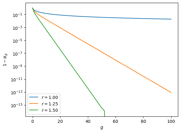
    (b) Plot \(1-\alpha_g\) for \(g = 1, \ldots, 100\) for these values of \(r\) with a logarithmic vertical scale. What unusual behavior do you see (if any)?

    Solution (b)

    See below. I should have given clearer guidance about the unusual behavior I was looking for. Interestingly the cases where \(\mu'(1)<1\) have a linear decay in this logarithmic scale while the case with \(\mu'(1)=1\) does not. This means that for \(\mu'(1)<1\) larger (but still finite) sizes are exponentially rare, while in the \(\mu'(1)=1\) case the larger sizes are rare, but not so rare. (in fact the average size in the \(\mu'(1)=1\) case is infinite, even though with probability 1 they all go extinct)

import matplotlib.pyplot as plt
import numpy as np

def mu(x,r): 
    return (r+(2-r)*x**2)/2
for r in [1, 5/4, 3/2]:
    alpha_g = [0]
    for g in range(1,101):
        alpha_g.append(mu(alpha_g[-1],r))
    plt.plot(1-np.array(alpha_g), label=rf"$r={r:.2f}$")
plt.figure(1)
plt.xlabel(r"$g$")
plt.ylabel(r"$1-\alpha_g$")
plt.semilogy()
plt.legend()
plt.show()

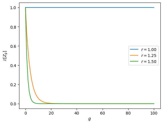
(c) Plot the expected size at generation \(g\) for these same values.

Solution (c)

See below

import numpy as np
def muPrime(x,r):
    return (2-r)*x
for r in [1, 5/4, 3/2]:
    expected_size = [1]
    for g in range(1,101):
        expected_size.append(muPrime(1,r)**g)
    plt.plot(expected_size, label=rf"$r={r:.2f}$")
plt.xlabel(r"$g$")
plt.ylabel(r"$\mathbb{E}[Z_g]$")
plt.legend()
plt.show()

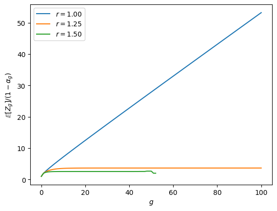
(d) Plot the expected size conditional on not being extinct.

Solution (d)

See below

for r in [1, 5/4, 3/2]:
    expected_size = [1]
    alpha_g = [0]
    for g in range(1,101):
        alpha_g.append(mu(alpha_g[-1],r))
        expected_size.append(muPrime(1,r)**g)
    plt.plot(np.array(expected_size)/(1-np.array(alpha_g)), label=rf"$r={r:.2f}$")
plt.xlabel(r"$g$")
plt.ylabel(r"$\mathbb{E}[Z_g]/(1-\alpha_g)$")
plt.legend()
plt.show()

C:\Users\JCMiller\AppData\Local\Temp\ipykernel_48448\3528766187.py:7: RuntimeWarning: divide by zero encountered in divide
  plt.plot(np.array(expected_size)/(1-np.array(alpha_g)), label=rf"$r={r:.2f}$")

12. [Optional] Consider a Galton-Watson process with an offspring PGF \(\mu(x)\), with \(\Phi_g(x)\) representing the PGF for \(X_g(t)\).

    (a) Define

    \[ \Psi_g(x) = \Phi_g(x) \frac{1}{1-x} \]

    Explain why \([x^k]\Psi_g(x)\) gives the probability that \(X_g \leq k\).

    Solution (a)

    As noted in the text, after multiplying by \(1/(1-x)\), the coefficient of \(x^k\) is equal to the sum of the coefficients \(a_0 + a_1 +\cdots + a_k\). So this is \(\sum_{j=0}^k p_j(g)\).

    (b) If we try to use

    \[ [x^k]\Psi_g(x) = \frac{1}{2\pi i} \oint_{|z|=1} \frac{\Psi_g(z)}{z^{k+1}} \, dz \]

    why will there be issues around \(z=1\)? Note - the initial version had a typo with the \(i\) missing from the denominator, and the wrong exponent on \(z\).

    Solution (b)

    Near \(z=1\), there is a singularity in \(\Psi_g(z)\).

    (c) Instead we will use the circle \(|z|=1/2\). Set \(z = e^{i\theta}/2\) for \(0 \leq \theta \leq 2\pi\). Rewrite the integral in terms of \(\theta\).

    Solution (c)

    We follow the text. Note that \(1 = i (e^{i\theta}/2) d\theta/dz\) so $dz = i (e^{i\theta}/2)d\theta

    \[\begin{align*} \frac{1}{2\pi i} \oint_{|z|=1/2} \frac{\Psi_g(z)}{z^{k+1}} \, dz &= \frac{1}{2\pi i} \int_0^{2\pi} \frac{\Psi_g(e^{i\theta}/2)}{e^{i(k+1)\theta}/2^{k+1}} \, \frac{ie^{i\theta}}{2} \, d\theta\\ &= \frac{2^{k-1}}{\pi} \int_0^{2\pi} \Psi_g(e^{i\theta}/2) e^{-ik\theta} \, d\theta \end{align*}\]

    (d) Adapt the method Phi_coefficients_real at https://github.com/Joel-Miller-Lab/AMSI2026_PGF/blob/main/AMSI_2026_PGF_tools/Galton_Watson.py and the methods it relies on to perform the integral above. Note that the code in place uses the Fast Fourier Transform by default, but I do not believe this will work for a radius of \(1/2\). So instead you will need to set it up to perform the integral. Ideally use Python or R.

    Solution (d)

    Time permitting I will add this solution later.

    (e) Choose a few simple offspring distributions and test the results.

    Solution ()