3.4. The Backward Kolmogorov Equation

The backward Kolmogorov equation along similar lines to the forward Kolmogorov equation. We assume we know \(\Phi(x,t)\) and \(\hat{\mu}(x)\) and we want to determine \(\Phi(x, t + \Delta t)\).

However, instead of taking the PGF for time \(t\), \(\Phi(x,t)\) and stepping forward an amount \(\Delta t\) using \(\hat{\mu}(x)\) as we did in deriving the Forward Kolmogorov Equations, we take the PGF for time \(\Delta t\) from Lemma 3.2 and step forward an amount \(t\) using \(\Phi(x,t)\). This will arrive at a different partial differential equation for \(\Phi(x,t)\). However, both equations will yield the same solution \(\Phi(x,t)\). Each equation gives insight into different properties of \(\Phi(x,t)\).

Given \(\Phi(x,0)= x\), that is, there is one individual at time \(t=0\), Lemma 3.2 tells us

\[ \Phi(x,\Delta t) = (1-r\Delta t)x + r\Delta t \hat{\mu}(x) \]

To determine \(\Phi(x,\Delta t + t)\), we now use Lemma 3.1 with \(T_1=\Delta t\) and \(T_2=t\). So

\[ \Phi(x,t+\Delta t) = (1-r\Delta t) \Phi(x,t) + r \Delta t \hat{\mu}(\Phi(x,t)) \]

This is illustrated in Fig. 3.6

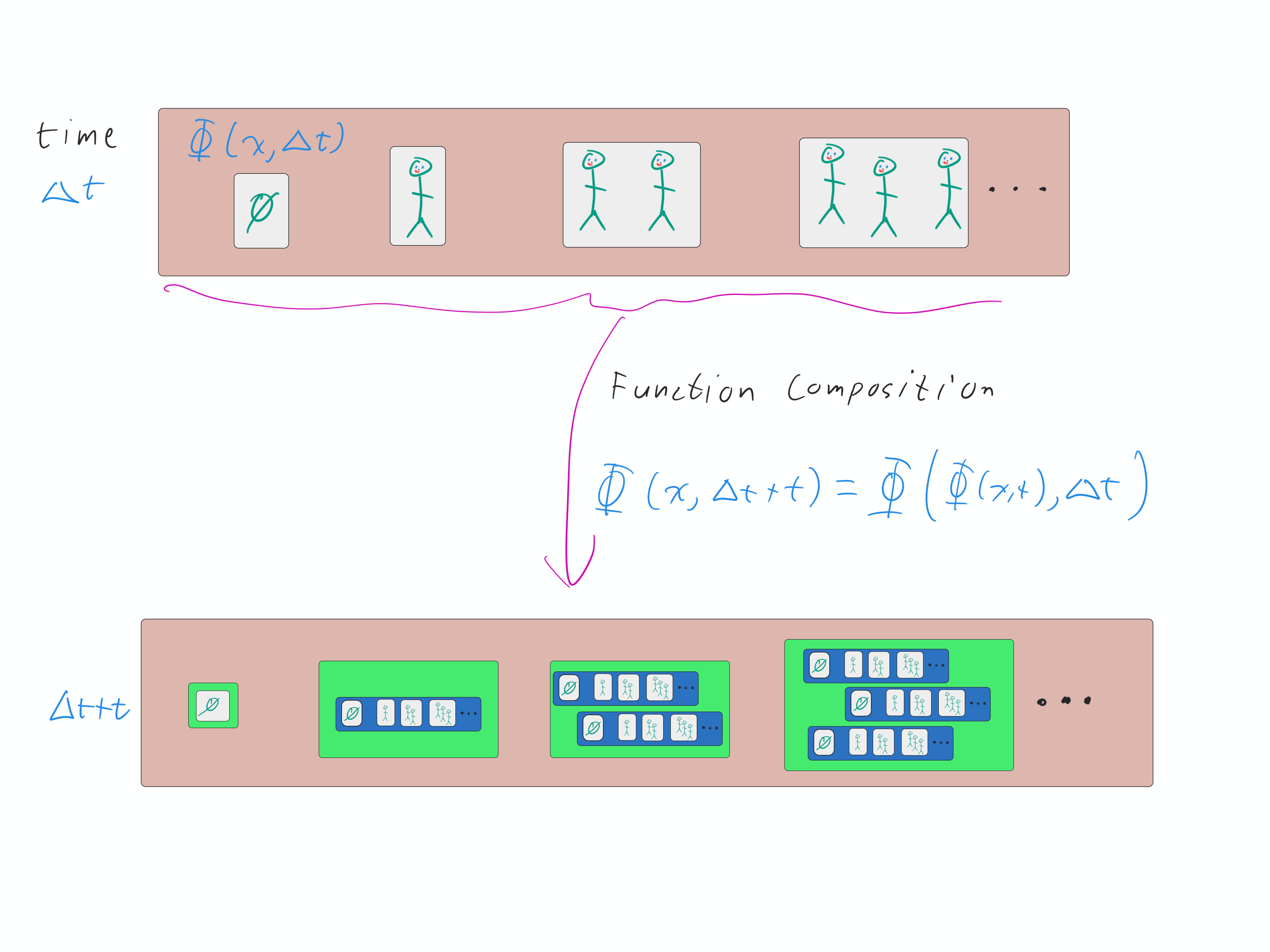
Fig. 3.6 Illustration of the derivation of \(\Phi(x,t+\Delta t)\) using function composition. We start from the PGF for \(X(\Delta t)\) and then step forward in time by a large amount \(t\). By Lemma 3.2 and Theorem 1.5, we substitute \(\Phi(x,t)\) for \(x\) in \(\Phi(x,\Delta t) = (1-r\Delta t)x + (r\Delta t)(\hat{\mu}(x))\). This yields \(\Phi(x,t+\Delta t) = (1-r\Delta t) \Phi(x,t) + r \Delta t \hat{\mu}(\Phi(x,t))\).

Calculating the \(t\) derivative of \(\Phi(x,t)\)

\[\begin{align*} \frac{\partial}{\partial t} \Phi(x,t) &= \lim_{\Delta t \to 0} \frac{\Phi(x,t+\Delta t)-\Phi(x,t)}{\Delta t}\\ &=\lim_{\Delta t \to 0} \frac{(1-r\Delta t) \Phi(x,t) + r \Delta t \hat{\mu}(\Phi(x,t)) - \Phi(x,t)}{\Delta t}\\ &= -r\Phi(x,t) + r \hat{\mu}(\Phi(x,t)) \\ &= r (\hat{\mu}(\Phi(x,t))-\Phi(x,t)) \end{align*} \]

This yields the Backward Kolmogorov Equation

\[ \frac{\partial}{\partial t} \Phi(x,t) = r (\hat{\mu}(\Phi(x,t))-\Phi(x,t)) \]

3.4.1. Extinction probability by time \(t\)

The probability of extinction by time \(t\) is \(\alpha(t) = q_{0}(t) = \Phi(0,t)\). The Backward Kolmogorov Equation gives

\[\begin{align*} \alpha'(t) &= \left[\frac{\partial}{\partial t} \Phi(x,t)\right]_{x=0}\\ &= r(\hat{\mu}(\Phi(0,t)-\Phi(0,t)))\\ &= r\left(\hat{\mu}(\alpha(t))-\alpha(t)\right) \end{align*}\]

with the initial condition \(\alpha(0)=0\).

If \(\hat{\mu}(0)=0\), then the extinction probability remains \(0\).

Otherwise, \(\hat{\mu}(0)>0\) and so initially \(\hat{\mu}\) is increasing. It continues to increase and it approaches the smallest value of \(x>0\) for which \(\hat{\mu}(x)=x\). This is the final extinction probability.

3.4.2. Self-test

1. We noted that if \(\hat{\mu}(0)=0\), then extinction is impossible. Under what conditions is \(\hat{\mu}(0)=0\)?

2. Define \(\alpha\) to be the eventual extinction probability. Following our derivation of \(\alpha\) in the generation-based case:

   (a) Explain why \(\alpha\) must be equal to the probability that when the first event happens, the individual either is removed or is replaced by \(k\) individuals, all of whom lead to eventual extinction.

   (b) Show that the explanation above implies \(\alpha = \hat{\mu}(\alpha)\).

   (c) Explain how we should address the case of multiple solutions to \(\alpha = \hat{\mu}(\alpha)\).