3.3. Forward Kolmogorov Equations

We now derive the Forward Kolmogorov equations which will tell us about how the PGF

\[ \Phi(x,t)= \sum_\ell q_\ell(t)x^\ell \]

changes in time.

We will work from the assumption that we know \(\Phi(x,t)\) and we will find \(\Phi(x,t+\Delta t)\). From this we will be able to determine the \(t\) derivative of \(\Phi\). For the forward Kolmogorov Equations, we mimic our (forward) approach for finding \(\Phi_g(x)\) in the generation-based approach. We start from the individuals in the population at time \(t\), and determine the PGF by stepping forward in time by \(\Delta t\) to derive \(\Phi(x,t+\Delta t)\), using \(\hat{\mu}\) and properties of PGFs.

3.3.1. Derivation

3.3.1.1. \(\Phi(x,t+\Delta t)\)

We first find \(\Phi(x,t+\Delta t)\).

We give two different derivations. The first is more elegant, but relies on Lemma 3.1 (which was proven using Theorem 1.5) and Lemma 3.2. The second is based on the same concept but revisits the method of derivation of Theorem 1.5 in a way that illustrates why an \(x\)-derivative of \(\Phi(x,t)\) arises.

First Derivation We will derive a partial differential equation for \(\Phi(x,t)\) by deriving \(\partial \Phi(x,t)/\partial t\).

To do this, we will find \(\Phi(x,t+\Delta t)\) and plug it into

\[ \frac{\partial}{\partial t} \Phi(x,t) = \lim_{\Delta t \to 0} \frac{\Phi(x,t+\Delta t) - \Phi(x,t)}{\Delta t} \]

By Lemma 3.1 with \(T_1=t\) and \(T_2 = \Delta t\), we can find \(\Phi(x,t+\Delta t)\) by plugging \(\Phi(x,\Delta t)\) into \(\Phi(x,t)\). From Lemma 3.2, we know \(\Phi(x,\Delta t) = x+ (r\Delta t)\left(\hat{\mu}(x)-x\right) + \mathcal{o}(\Delta t)\). So we get

\[ \Phi(x,t+\Delta t)= \Phi\left(x + (r\Delta t) \left(\hat{\mu}(x)-x\right)+\mathcal{o}(\Delta t), t\right) \]

Then using some Algebra and a Taylor Series expansion in \(x\):

\[\begin{align*} \Phi(x,t+\Delta t)&= \Phi\left(x + (r\Delta t) \left(\hat{\mu}(x)-x\right)+\mathcal{o}(\Delta t), t\right)\\ &= \Phi(x,t) + (r\Delta t+\mathcal{o}(\Delta t))\left(\hat{\mu}(x)-x\right) \frac{\partial}{\partial x}\Phi(x,t) + \mathcal{o}(\Delta t)\\ &= \Phi(x,t) + (r\Delta t)\left(\hat{\mu}(x)-x\right) \frac{\partial}{\partial x}\Phi(x,t) + \mathcal{o}(\Delta t) \end{align*}\]

This is illustrated in Fig. 3.4

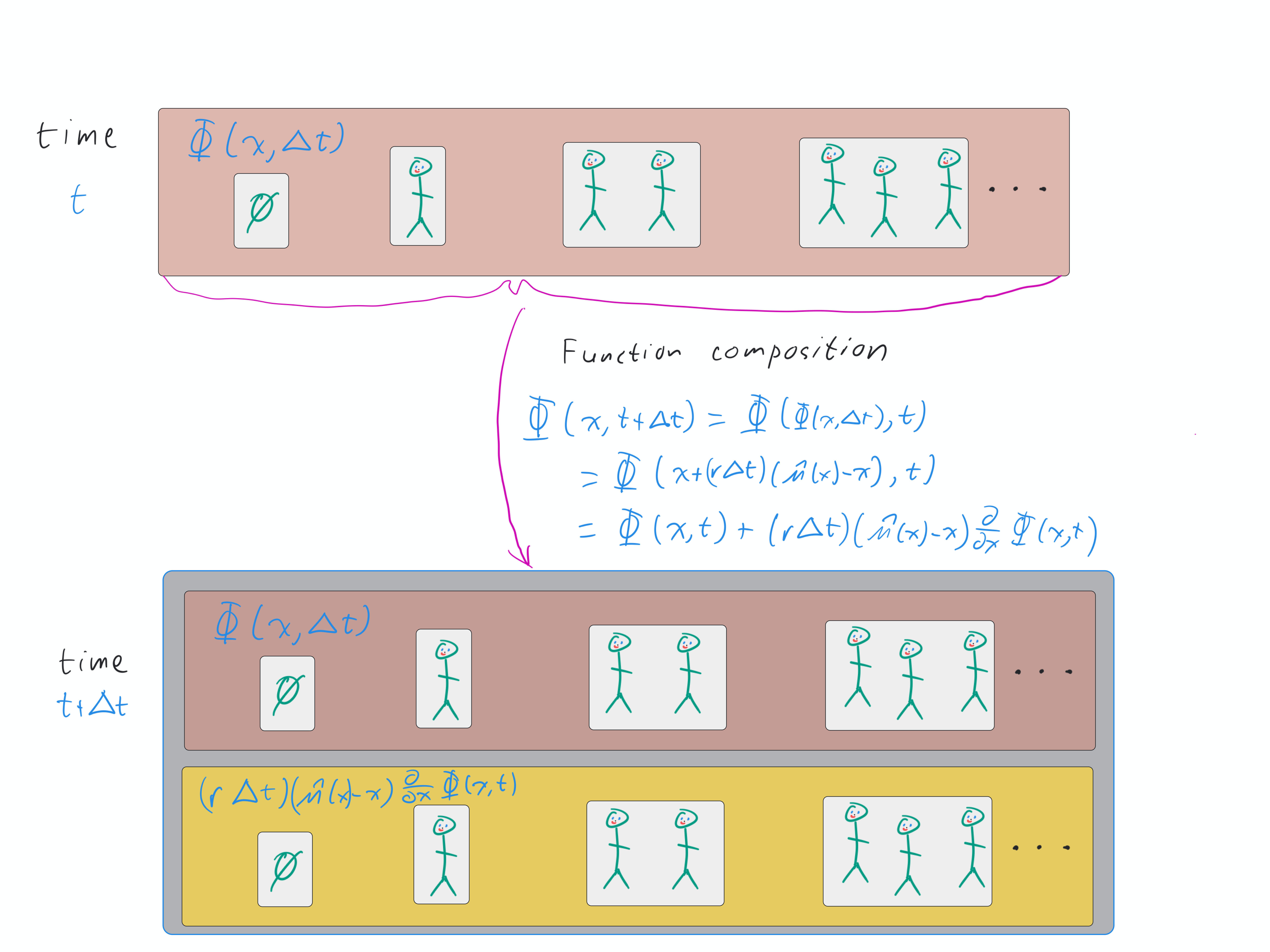
Fig. 3.4 Illustration of the first derivation of \(\Phi(x,t+\Delta t)\) (leaving out neglected terms). We start from the PGF for \(X(t)\) and then step forward in time by a small amount \(\Delta t\). By Lemma 3.1, we substitute \(\Phi(x,\Delta t)=x + (r\Delta t) (\hat{\mu}(x)-x)\) for \(x\) in \(\Phi(x,t)\). Then expanding \(\Phi\) using the Taylor Series, we find \(\Phi(x,t+\Delta t) = \Phi(x,t) + (r\Delta t) (\hat{\mu}(x)-x) \frac{\partial }{\partial x} \Phi(x,t)\).

Second Derivation (in this derivation we will not track the \(\mathcal{o}(\Delta t)\) terms)

If there are known to be exactly \(X(t)=\ell\) individuals at time \(t\), then we can consider the Poisson process created from the superposition of the Poisson processes for each individual. The combined rate is \(\ell r\). The probability that an event happens in the next \(\Delta t\) units of time can be treated as \(\ell r \Delta t\) for \(\Delta t \ll 1\). When the first event occurs, one random individual is removed and replaced with \(k\) individuals, chosen from the distribution corresponding to \(\hat{\mu}(x)\). The PGF of the resulting population at time \(t+\Delta t\) is \(x^{\ell-1} \hat{\mu}(x)\).

So again assuming we know \(X(t)=\ell\), but now assuming we do not know whether an event will occur in the interval \([t,t+\Delta t)\), the PGF for \(X(t+\Delta t)\) is given by the convex combination of the PGFs if nothing happens and the PGF if an event happens. This is (approximately as \(\Delta t \to 0\))

\[ (1-\ell r\Delta t) x^\ell + \ell r (\Delta t) x^{\ell-1}\hat{\mu}(x) \]

This is illustrated in Fig. 3.5

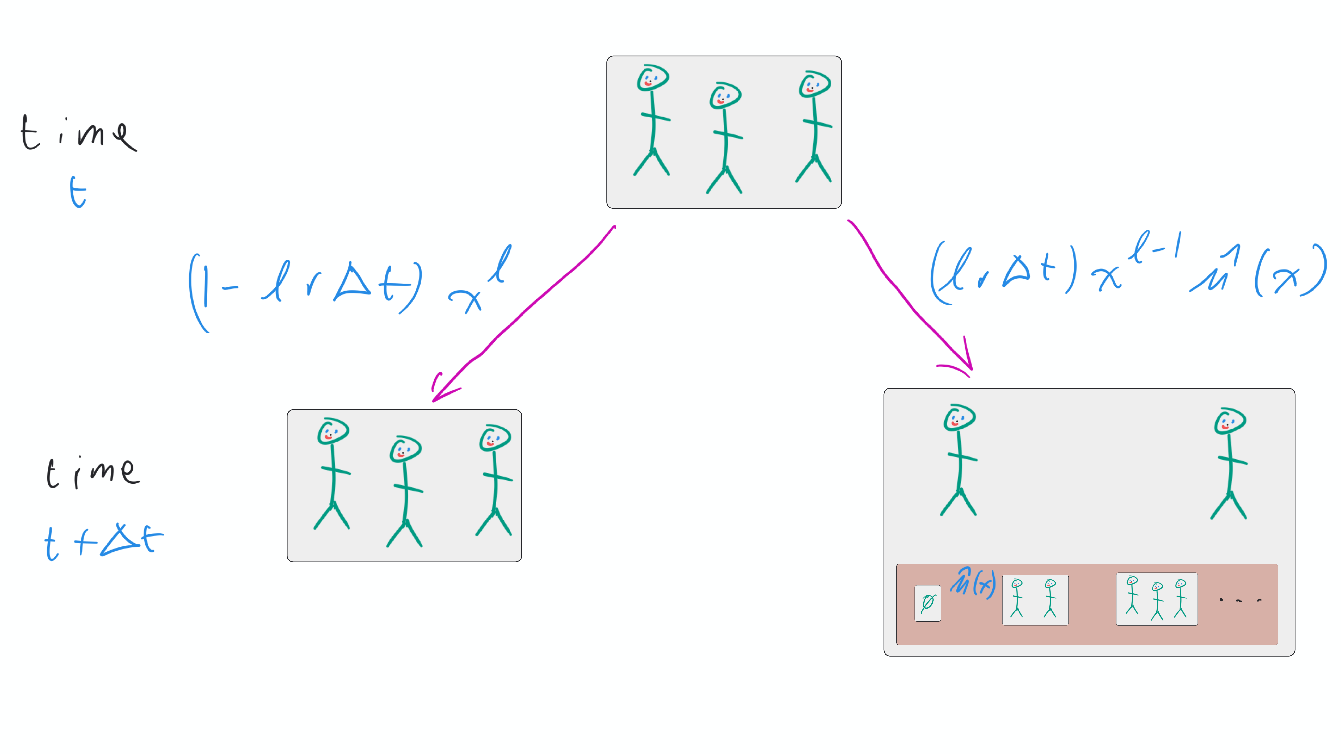
Fig. 3.5 Illustration of one step of the second derivation of \(\Phi(x,t+\Delta t)\). If we know that \(X(t)=\ell\), then at time \(t+\Delta t\), the probability none of them have changed is \(1-\ell r\Delta t\), leaving a PGF of \(x^\ell\). The probability that one changes is \(\ell r \Delta t\) leaving a PGF of \(x^{\ell-1} \hat{\mu}(x)\). Adding these two gives the PGF at time \(t+\Delta t\) if we know \(\ell\). Summing over all \(\ell\) gives the PGF at time \(t+\Delta t\) if we only know the distribution of \(\ell\).

Now using the rule for convex combinations of PGFs we can find the PGF of \(X(t+\Delta t)\) if we only know the probability \(q_{\ell}(t)\) that \(X(t)=\ell\):

\[\begin{align*} \Phi(x, t+\Delta t) &= \sum_\ell q_{\ell}(t) \left((1-\ell r\Delta t) x^\ell + \ell r \Delta t x^{\ell-1}\hat{\mu}(x)\right)\\ &=\sum_\ell q_{\ell}(t) x^\ell + (r\Delta t) \sum_{\ell} q_\ell(t) \ell (x^{\ell-1}\hat{\mu}(x) - x^{\ell})\\ &= \Phi(x,t) + (r\Delta t) \hat{\mu}(x)\sum_{\ell}\frac{\partial}{\partial x} q_\ell(t) x^\ell - (r \Delta t) \sum_\ell \ell q_\ell(t) x^\ell\\ &=\Phi(x,t) +(r \Delta t) \hat{\mu}(x) \frac{\partial}{\partial x} \Phi(x,t) - (r \Delta t) x \frac{\partial}{\partial x} \Phi(x,t) \end{align*}\]

(technically there are some error terms in the above which are \(\mathcal{o}(\Delta t)\) that have been neglected).

3.3.1.2. Finding \(\partial \Phi(x,t)/\partial t\)

Using the definition of the derivative:

\[\begin{align*} \frac{\partial}{\partial t} \Phi(x,t) &= \lim_{\Delta t \to 0} \frac{\Phi(x,t+\Delta t) - \Phi(x,t)}{\Delta t}\\ &= \lim_{\Delta t \to 0}\frac{\Phi(x,t) + r \Delta t \hat{\mu}(x) \frac{\partial}{\partial x} \Phi(x,t) - r \Delta t x \frac{\partial}{\partial x} \Phi(x,t) +\mathcal{o}(\Delta t)- \Phi(x,t)}{\Delta t}\\ &= r \hat{\mu}(x) \frac{\partial}{\partial x} \Phi(x,t) - r x \frac{\partial}{\partial x} \Phi(x,t)\\ &= r(\hat{\mu}(x)-x) \frac{\partial}{\partial x} \Phi(x,t) \end{align*}\]

This yields

Theorem 3.4 (Forward Kolmogorov Equation)

The PGF \(\Phi(x,t)\) for \(X(t)\) satisfies the Forward Kolmogorov Equation

\[ \frac{\partial}{\partial t} \Phi(x,t) = r (\hat{\mu}(x)-x) \frac{\partial}{\partial x} \Phi(x,t) \]

with initial condition \(\Phi(x,0)=x\).

Example 3.4 (A pure birth process)

Assume individuals give birth to a single individual with rate \(\beta\). Further assume that they never die. In our context when they give birth, this is equivalent to replacing them by two indviduals. Here \(r=\beta\) and \(\hat{\mu}(x)=x^2\), and \(\Phi(x,0)=x\). We have

\[ \frac{\partial}{\partial t} \Phi(x,t) = r (x^2-x) \frac{\partial}{\partial x} \Phi(x,t) \]

It can be shown that the solution to this equation is

\[ \Phi(x,t) = \frac{x e^{-rt}}{1-(1-e^{-rt})x} \]

Expanding this using a geometric series

\[\begin{align*} \Phi(x,t) &= x e^{-rt} \sum_{n=0}^\infty (1-e^{-rt})^n x^n\\ &= \sum_{n=0}^\infty e^{-rt}(1-e^{-rt})^n x^{n+1}\\ &= \sum_{\ell=1}^\infty e^{-rt} (1-e^{-ert})^{\ell-1} x^\ell \end{align*}\]

So the probability of \(\ell\) individuals is \(q_{\ell}(t) = e^{-rt} (1-e^{-ert})^{\ell-1}\)

3.3.2. Expected Population size

Let \(L(t)\) denote the expected size of the population at time \(t\). Then \(L(t) = \left[ \frac{\partial}{\partial x} \Phi(x,t) \right]_{x=1}\) and

\[\begin{align*} \frac{d}{dt}L(t) &= \frac{\partial}{\partial t} \left[\frac{\partial}{\partial x} \Phi(x,t) \right]_{x=1}\\ &= \left[\frac{\partial}{\partial x} \frac{\partial}{\partial t} \Phi(x,t) \right]_{x=1}\\ &= \left[\frac{\partial}{\partial x} \left(r(\hat{\mu}(x)-x) \frac{\partial}{\partial x} \Phi(x,t)\right)\right]_{x=1}\\ %&= r (\hat{\mu}'(1)-1) L(t) + r(\hat{\mu}(1)-1)\frac{\partial^2}{\partial x^2} \Phi(1,t)\\ &= r (\mu'(1)-1)L(t) + r (1-1) \frac{\partial^2}{\partial x^2} \Phi(1,t)\\ &= r (\mu'(1)-1)L(t) \end{align*}\]

The next to last step uses the product rule and substitutes \(1\) for \(x\). The last step uses the fact that \(\hat{\mu}(1)=1\).

The solution to this differential equation is \(L(t) = L(0)\exp(ct)\) where \(c=r(\hat{\mu}'(1)-1)\). Note that For our assumptions \(L(0)=1\).

So \(L(t)\) grows or decays exponentially depending on the value of \(r(\hat{\mu}'(1)-1)\). If on average the individuals are replaced with fewer than \(1\) individual \(\hat{\mu}'(1)-1<0\) and decay occurs, while if \(\hat{\mu}'(1)-1>0\) growth occurs.

So we have seen that the expected population size in a continuous-time Galton-Watson process is exponential with growth rate \(r(\hat{\mu}'(1)-1)\).

Definition 3.7 (Malthusian Parameter)

The expected size of a continuous-time Galton-Watson process is \(e^{r(\hat{\mu}'(1)-1)t}\). The parameter \(r(\hat{\mu}'(1)-1)\) which governs the growth is the Malthusian Parameter.

3.3.3. Self-test

1. The text claims that when an event happens in a population of \(\ell\) individuals the PGF after the event is \(x^{\ell-1} \hat{\mu}(x)\). Justify this claim.

2. Use the Forward Kolmogorov Equation for the PGF \(\Phi(x,t)\) to find a system of equations for \(\frac{d}{d t} q_\ell(t)\) for each \(\ell\). This system is often called the master equation as well as also being called the Forward Kolmogorov Equations.

3. Consider the case where individuals give birth at rate \(\beta\) and die at rate \(\gamma\).

   (a) Derive the Forward Kolmogorov Equation.

   (b) Find the Malthusian Parameter.

   (c) What is the initial condition for \(\Phi(x,0)\)?

   (d) Show that if \(\gamma \neq \beta\)

   \[ \Phi(x,t) = \frac{(\gamma-\beta x)e^{-(\beta-\gamma)t} - \gamma(1-x)}{(\gamma-\beta x)e^{-(\beta-\gamma)t}-\beta(1-x)} \]

   is a solution (you don’t need to derive it, just show that it satisfies the equation).

   (e) Find \(q_0(t) = \Phi(0,t)\) (if \(\beta \neq \gamma\)).

   (f) If \(s(t) = \frac{\beta(1-e^{-(\beta-\gamma)t})}{\beta-\gamma e^{-(\beta-\gamma)t}}\) then

   \[ \Phi(x,t) = q_0(t) + (1-q_0(t)) \frac{(1-s(t))x}{1-s(t)x} \]

   (you do not need to show this). Based on this, find \(q_\ell(t)\) for \(\ell=1,2,\ldots\) in terms of \(q_0(t)\) and \(s(t)\).

4. Define \(\hat{\Phi}(\theta,t) = \Phi(e^{i\theta},t)\).

   1. Convert the Kolmogorov Forward Equation into an equation with \(t\) and \(\theta\) derivatives for \(\hat{\Phi}\).

   2. Determine the initial condition \(\Phi(\theta, 0)\).

   3. Assume we can solve this system of equations numerically for \(\theta = 2\pi m/M\) for \(m=1,\ldots, M\). Explain how we could find \(q_\ell(t)\).

5. Consider trying to find the extinction probability \(\alpha(t) = \Phi(0,t)\) from the (PGF formulation of the) Forward Kolmogorov Equation. For simplicity of notation, define the time-dependent coefficients \(p_k(t) = \mathbb{P}[X(t)=k]\) so that \(\Phi(x,t) = \sum_{k=0}^\infty p_k(t) x^k\). Take \(\hat{\mu}(x) = q_0 + q_2 x^2\).

   (a) Show that you can find \(\frac{d}{dt}\alpha(t)=\frac{d}{dt} p_0(t)\) in terms of \(\frac{\partial}{\partial x} \Phi(0,t)\), and express this in terms of \(p_1(t)\).

   (b) Now similarly find \(\frac{\partial}{\partial t} \frac{\partial}{\partial x} \Phi(0,t)\) and use it to express \(\frac{d}{dt} p_1(t)\) in terms of other \(p_k(t)\).

   (c) Explain how you could use this to find an (infinite) system of ordinary differential equations for \(p_k(t)\). This system is called the “master equation” or “master equations”, and often it is referred to as the “Forward Kolmogorov Equation”.