The Galton-Watson Process

2. The Galton-Watson Process#

2.1. Introduction#

One of the first applications of Probability Generating Functions in biological contexts was by Galton and Watson in the mid 1860s and 1870s. They were concerned about the extinction of aristrocratic family names in England, where the names were passed down from father to sons. Others independently introduced the Galton-Watson process both before and after Galton and Watson.

To investigate the probability a name goes extinct, we start by analyzing one male individual and consider sons he might have. Assume that each male has $k$ male offspring with probability $p_k$ and they all inherit the family name. We call the distribution of the number of male offspring the offspring distribution. We assume that the offspring distribution remains the same from generation to generation.

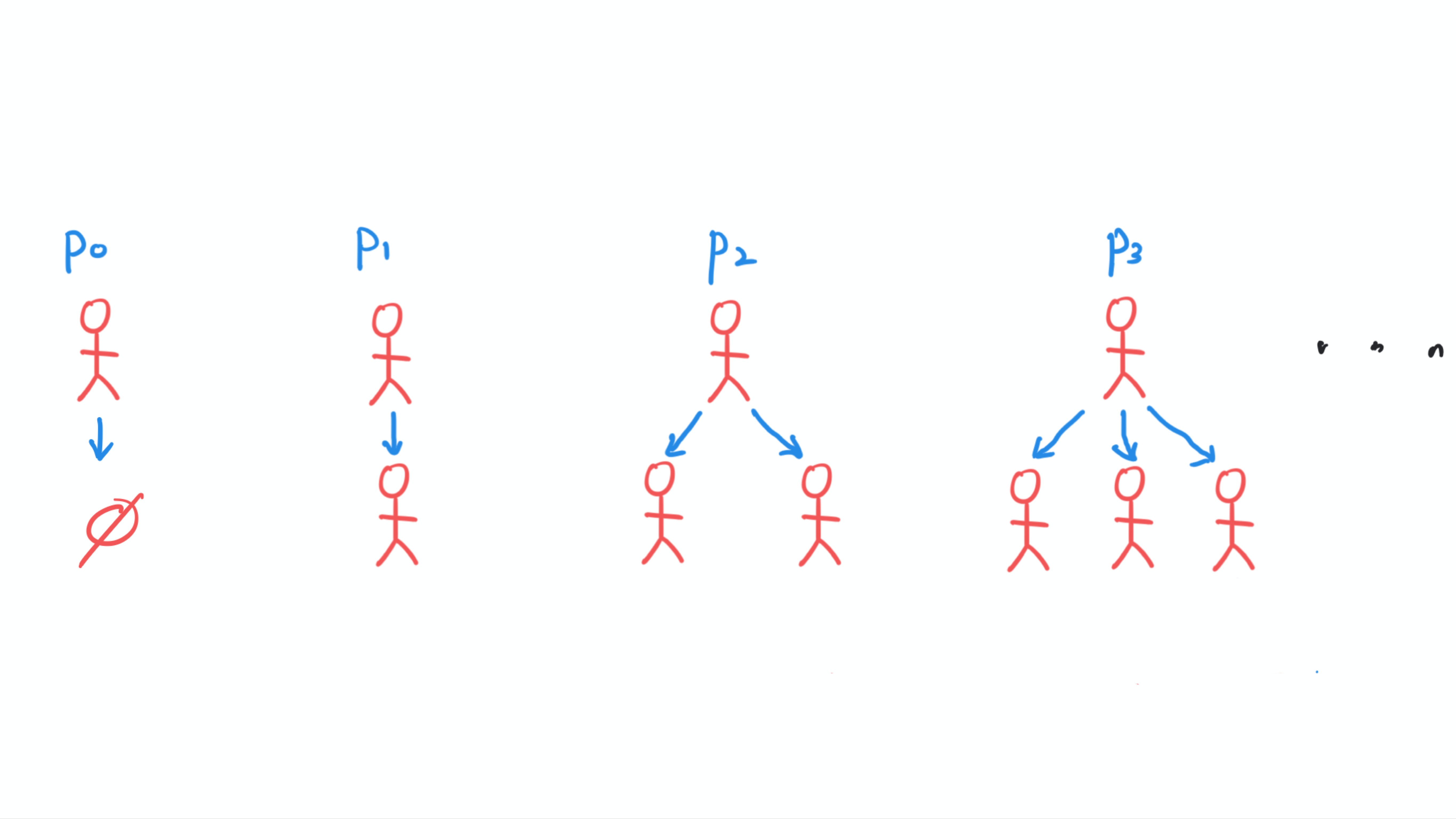
../../_images/OffspringDist.png — Fig. 2.1 An illustration of an offspring distribution.#

Definition 2.1 (The Galton-Watson Process)

Consider a distribution of non-negative integers where $p_k$ is the probability of $k$, which we call the offspring distribution. A Galton-Watson process is a sequence of random numbers $\{X_g\}_{g \in \mathbb{N}}$ such that $X_0=1$ and $X_{g+1} = \sum_{j=1}^{X_g} k_{g,j}$ where each $k_{g,j}$ is chosen independently from the offspring distribution. The numbers are indexed by generation $g$.

In the family name context, $X_g$ is the number of male descendants at generation $g$, and $k_{g,j}$ is the number of male offspring of the $j$’th male descendant at generation $g$.

An example of the first few steps of a Galton-Watson Process is the sequence as follows:

\[\begin{align*} X_0 &= 1 \qquad \qquad \qquad \qquad &&k_{0,1}= 1\\ X_1 &= 1 \qquad \qquad \qquad \qquad &&k_{1,1}= 3\\ X_2 &= 3 \qquad \qquad \qquad \qquad &&k_{2,1}= 2, \: k_{2,2} = 0, \: k_{2,3} = 1\\ X_3 &= 3 \qquad \qquad \qquad \qquad &&k_{3,1}= 2, \: k_{3,2} = 2, \: k_{3,3} = 3\\ X_4 &= 7 \qquad \qquad \qquad \qquad &&\cdots \end{align*}\]

Conceptually, each of the $X_g$ individuals is indexed by $j$ and has $k_{g,j}$ offspring.

2.1.1. Galton-Watson Trees#

Conceptually, we often think of a Galton-Watson process as consisting of individuals who are alive for one generation and at the end of generation $g$, the $j$th individual of that generation is replaced by their offspring: $k_{g,j}$ new individuals where $k_{g,j}$ is chosen from the offspring distribution. The “parent-child” relationship leads naturally to a directed tree whose root is the initial individual.

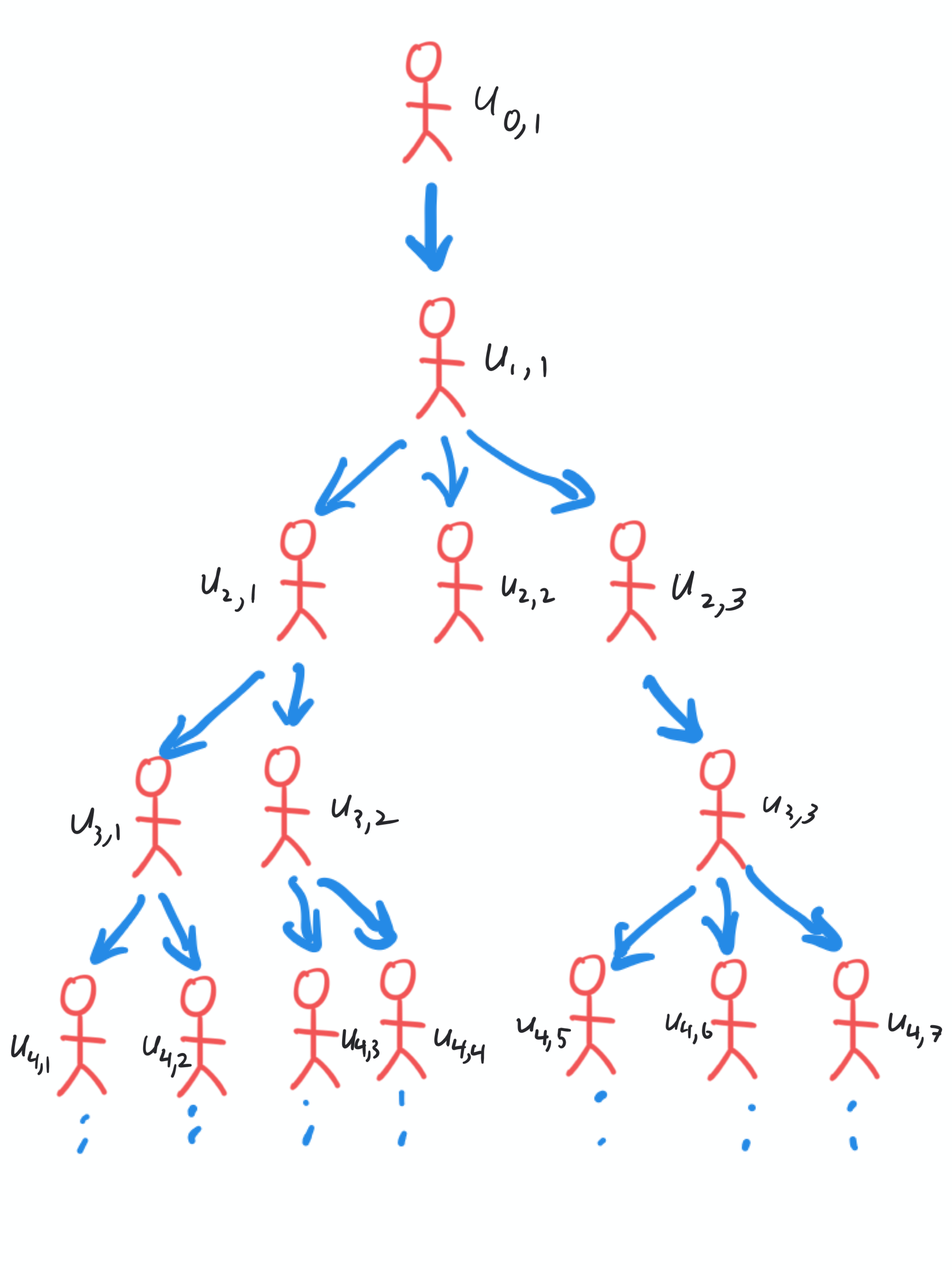
../../_images/ExampleGaltWatLabelled.png — Fig. 2.2 An illustration of generations $0$ to $4$ in a Galton-Watson tree.#

This leads to an equivalent description of a Galton-Watson process through a directed tree, which we call a Galton-Watson tree. Often it will be easier to prove things about the set of Galton-Watson trees rather than the sequence of numbers $\{X_g\}$.

The tree shown in Fig. 2.2 is an example of a Galton-Watson tree. Now we give a formal definition of how to create one, starting from the top node and building each level by choosing the number of “offspring” of each node from the offspring distribution. We choose to index the nodes $u_{g+1,j}$ in level $g+1$ so that their order follows the ordering of their “parents”.

Definition 2.2 (Galton-Watson tree)

Consider the directed tree formed from a given offspring distribution by the following process:

Create a single node, labelled $u_{0,1}$ and set $X_0=1$.
Choose $k_{0,1}$ from the offspring distribution, and create nodes $u_{1,1}, u_{1,2}, \ldots, u_{1,k_{0,1}}$, with a directed edge from $u_{0,1}$ to each of these nodes. Set $X_1 = k_{0,1}$.
Construct the remaining tree iteratively for each $g \geq 1$ by assigning each node $u_{g,j}$ a number $k_{g,j}$ chosen from the offspring distribution. Define $n_j = \sum_{\ell=0}^j k_{g,\ell}$. Then create the nodes $u_{g+1,n_{j-1}+1}, u_{g+1,n+1}, \ldots, u_{g+1, n_j}$ with an edge from $u_{g,j}$ to each of them. Set $X_{g+1} = \sum_{j=1}^{X_{g}} k_{g,j}$.

The resulting tree may be infinite.

Definition 2.3 (Offspring, descendent, parent, ancestor, root, generation)

The nodes that $u_{g,j}$ points to are referred to as its offspring.
The nodes that are reachable from $u_{g,j}$ following the edge directions are its descendents.
For $g>0$, the node that has an edge to $u_{g,j}$ is its parent.
The nodes that are reachable from $u_{g,j}$ following edges in reversed order are its ancestors.
The node $u_{0,1}$ is called the root.
The number of edges in the path from $u_{0,1}$ to $u_{g,j}$ is $g$, known as the generation of $u_{g,j}$.

Theorem 2.1 (Galton-Watson trees are Galton-Watson processes.)

Given a Galton-Watson tree, the sequence of numbers $\{X_g\}$, where $X_g$ is the number of nodes in generation $g$, forms a Galton-Watson process. Similarly, every Galton-Watson process can be represented by a Galton-Watson tree.

To prove this, we show that the definition of a Galton-Watson process Definition 2.1 is satisfied.

We must show that the number of nodes $X_g$ in generation $g$ is a sequence of random numbers $\{X_g\}_{g \in \mathbb{N}}$ such that $X_0=1$ and $X_{g+1} = \sum_{j=1}^{X_g} k_{j,g}$ where each $k_{j,g}$ is chosen independently from the offspring distribution.

Proof. We just have to check that the conditions of a Galton-Watson process are satisfied.

The fact that $X_0=1$ follows from the assumption of a single root.
For each of the $X_g$ infected nodes in generation $g$, the number of offspring is chosen independently from the offspring distribution. Thus $X_{g+1} = \sum_{j=1}^{X_g} k_{j,g}$ where $k_{j,g}$ is chosen independently from the offspring distribution.

Thus the definition of a Galton-Watson process is satisfied.

2.1.2. Applications of the Galton-Watson Process#

Although the focus on family names is perhaps frivolous, there are many other important scenarios that are mathematically equivalent. For example:

An invasive species has arrived at a location. Each female produces $k$ female offspring with probability $p_k$.
A virus has just entered a person’s body and begins to infect cells. Each virus produces $k$ new viruses with probability $p_k$.
An infected individual has just entered a large population. Each infected individual creates $k$ new infections with probability $p_k$.
A cell has just mutated to become cancerous. Each cancerous cell produces $k$ new cells with probability $p_k$ (in this case the cell either dies $k=0$ or divides $k=2$).
A new mutated gene appears in a single individual which may have beneficial or harmful effects. These are passed down to its offspring.
A gambler buys a $1 lottery ticket. The ticket pays $k with probability $p_k$. The gambler spends all proceeds on new $1 tickets (with the same probabilities $p_k$).

2.1.3. Self-test#

Consider a Galton-Watson process whose offspring distribution has $\mathbb{P}(k=3)=1$, that is, all individuals have $3$ offspring.
1. Draw the corresponding Galton-Watson Tree up to (and including) generation $2$.
2. Label each node.
3. What is the sequence $\{X_g\}$?
4. Explain why for each $g$ and $j$, the subset of the tree made up by $u_{g,j}$ and its descendents forms a Galton-Watson tree.
Convince yourself that each example in Section 2.1.2 is a Galton-Watson Process.