Assignment 2

8.2. Assignment 2#

This will be ~~due Saturday 31 Jan, 11:59PM~~ due Sunday 1 Feb 11:55PM. I’ll set up a submission portal on Moodle.

If you get help or give help to anyone else, please find a similar problem to discuss. Do not directly work on a problem in the question.

These problems are not ordered by difficulty. They are ordered roughly with where the corresponding material appears in the text. I have a reputation for setting long assignments (I get excited by what each problem can reveal to students). I will have consultation hours (and I will make sure that you can reach me on zoom if you are remote). As I see where people struggle, I may add hints to these questions.

8.2.1. Instructions for AI use:#

Never trust anything that can think for itself if you can’t see where it keeps its brain.

— Arthur Weasley, Harry Potter and the Chamber of Secrets

AI can be an amazing learning tool. It is also amazingly effective at preventing learning. There is a lot of benefit in looking at a problem on your own, thinking about how to solve it, and even running into dead-ends when you attempt the wrong method.

Here are the guidelines for use of AI on this problem set:

Before turning to AI for assistance on a question, think about the question yourself. Identify what the question is asking and make some attempt to solve it on your own.
If you use an AI, you must save the “conversation” you have.
You must start the conversation with the prompt below, and you cannot encourage the AI to violate the prompt.
You must complete the “Learning Reflection” below for each question on which you used AI.

8.2.1.1. AI Prompt#

I am working on a problem that I must solve on my own. Please do not give me the full solution. Instead:

Find a similar problem to solve.
Ask me questions to check whether I understand each step.
Only reveal the next step after I attempt it.
If I make a mistake, respond with hints instead of the correct answer.

My goal is to understand and be able to solve similar problems without AI.

8.2.1.2. Learning Reflection#

What did I already know about this problem before asking AI?
What did I learn?
What detail or technique was the most important for completing this problem?

(3-6 sentences maximum)

8.2.2. Problem set#

Any edits since the assignment was released are in bold

(29 Jan 4pm) I screwed up a correction. Please attempt Q5 and not Q4. Follow the derivation of the expected size given in the forward kolmogorov section of the notes for Q5. On Q3, do not attempt the backward Kolmogorov part

Let us assume we are waiting for some event (e.g., death of a single bacterium or a red light turning green). We make the assumption that if the event hasn’t happened prior to time \(t\), then for any fixed \(\Delta t\), the probability that it occurs between \(t\) and \(t+\Delta t\) is the same for any \(t\). This means that we assume that the knowledge of how long it has “survived” so far does not give us any extra information. In other words, we are making the assumption that the distribution is memoryless. Our goal in this question is to show that memoryless distributions must have an exponential waiting time distribution. Please do not assume that this is a Poisson process or that it has an exponential waiting time distribution to do this question.

(a) Let \(s(t)\) denote the probability that it has survived to time \(t\), with \(s(0)=1\). Show that \(s(t_0+t_1) = s(t_0)s(t_1)\) for any positive \(t_0\) and \(t_1\).

Solution (a)

There are multiple ways to do this. Let’s find a \(\Delta t\) which is very small such that \(t_0 = N \Delta t\) and \(t_1 = M \Delta t\) Implicitly, I’m assuming that \(t_0/t_1\) is rational — this can be patched up by taking an arbitrariliy good approximation to \(t_0\) such that the ratio is rational. (As an aside, this is why the Pythagorean theorem caused Greeks such trouble — they had assumed that this could be done with any pair of lengths, so they could prove things about similar triangles by using this assumption. They knew that \(\sqrt{2}\) wasn’t rational, but they could simply assume that there was no such length. Suddenly the Pythagorean theorem gave them a way to create that length, and so their old proofs were flawed.)

Then if \(p\) is the probability it would occur in a given interval of length \(\Delta t\) the probability of no event in the entire interval is \(s(t_0+t_1)=(1-p)^{(N+M)} = (1-p)^N (1-p)^M = s(t_0)s(t_1)\).

(b) Consider a Taylor Series expansion for \(s(t)\). Use this to explain why for small \(\Delta t\), we can approximate \(s(\Delta t) = 1 - r \Delta t + \mathcal{o}(\Delta t)\).

Solution (b)

There are multiple options for how to do this.

We simply observe that \(s(0)\) must equal \(1\) and then write out the Taylor Series expansion which states that \(s(\Delta t) = 1 - r\Delta t + \mathcal{o}(\Delta t)\).

(c) Use the definition of a derivative to derive an equation for \(ds/dt\).

Solution (c)

\[\begin{align*} \frac{d}{dt} s(t) &= \lim_{\Delta t \to 0} \frac{s(t+\Delta t)-s(t)}{\Delta t}\\ &= \lim_{\Delta t \to 0} \frac{s(t)s(\Delta t) - s(t)}{\Delta t} \\ &= \lim_{\Delta t \to 0} \frac{s(t)(1 + r\Delta t + \mathcal{o}(\Delta t)) - s(t)}{\Delta t}\\ &= \lim_{\Delta t \to 0} \frac{ -s(t) r\Delta t + s(t) \mathcal{o}(\Delta t)}{\Delta t}\\ &= -s(t) r \end{align*}\]

(d) Find the solution for \(s(t)\).

Solution (d)

if \(ds/dt = -rs\), then \(s = s(0) e^{-rt}\). In this case \(s(0)=1\), so \(s(t) = e^{-rt}\).

(e) What can we conclude about \(s(t)\) if the distribution is memoryless?

Solution (e)

If the distribution is memoryless, then \(s(t)\) must be \(e^{-rt}\) for some (non-negative) constant \(r\).
Consider a continuous-time Galton-Watson process in which individuals are removed with rate \(r\) and when they are removed they are replaced by \(k\) individuals with probability \(p_k\). Define \(r_k = r p_k\) for \(k = 0, 1, \ldots\) (we could assume \(r_1=p_1=0\), but this is not necessary here)

(a) Use the principle of superposition of Poisson processes to explain why this is equivalent to saying that for \(k = 0, 1, \ldots\) an individual is removed at rate \(r_k\) and replaced with \(k\) individuals.

Solution (a)

If we consider that for \(k=0, 1, \ldots\) an individual is removed at rate \(r_k\) and replaced with \(k\) individuals, then by superposition, the Poisson process having rate \(r = \sum_k r_k\) and then selecting \(k\) with probability \(r_k/r\) must be equivalent.

But that is exactly the process we are considering. So effectively we have simply shown that what we are studying is equivalent to superposition of the different \(k\)-processes.

(b) In terms of the rates \(r_k\), write down the probability of a specific individual being replaced by \(k\) individuals in a short time interval of length \(\Delta t\).

Solution (b)

\(r_k \Delta t\).

(c) If there are \(X(t)\) individuals, write down the probability that one of them is replaced by \(k\) individuals in a short time interval of length \(\Delta t\).

Solution (c)

\(X(t) r_k \Delta t\)
Consider the continuous-time Galton-Watson process with offspring distribution \(\hat{\mu}(x)\) and associated rate \(r\) per individual.

(a) Find the initial condition for \(\Phi(x,t)\) if \(X(0)=2\) with probability \(1\).

Solution (a)

\[ \Phi(x,0) = \sum_k \mathbb{P}[X=k]x^k = x^2 \]

(b) Find the Forward Kolmogorov Equations if \(X(0)=2\).

Solution (b)

\(\Phi(x,t)\) is the PGF for time \(t\). Let \(X(t)\) be the random number present at time \(t\).

The random number present at time \(t+\Delta t\) is most easily found by noting that the PGF for the number of descendents of a single individual after waiting a time \(\Delta t\) is a random number (say, \(M\)) whose PGF is \((1-r\Delta t)x + r\Delta t \hat{\mu}(x) = x + r\Delta t(\hat{\mu}(x)-x)\).

We need to add up \(M_i\) for each of the \(i=1,2,\ldots, X(t)\) individuals at time \(t\). This is a randomly stopped sum. By Theorem 1.5 the PGF for the sum is \(\Phi(x + r\Delta t(\hat{\mu}(x)-x), t)\), but by definition it is also \(\Phi(x,t+\Delta t)\). Expanding this around \(x\), we have

\[\begin{align*} \Phi(x, t+\Delta t) &= \Phi(x + r\Delta t(\hat{\mu}(x)-x), t)\\ &= \Phi(x, t) + r \Delta t (\hat{\mu}(x)-x) \frac{\partial}{\partial x} \Phi(x,t) \end{align*}\]

Now finding the time derivative:

\[\begin{align*} \frac{\partial}{\partial t} \Phi(x,t) &= \lim_{\Delta t \to 0} \frac{\Phi(x,t+\Delta t) - \Phi(x,t)}{\Delta t}\\ &= \lim_{\Delta t \to 0} \frac{\Phi(x, t) + r \Delta t (\hat{\mu}(x)-x) \frac{\partial}{\partial x} \Phi(x,t) - \Phi(x,t)}{\Delta t}\\ &= \lim_{\Delta t \to 0} \frac{ r \Delta t (\hat{\mu}(x)-x) \frac{\partial}{\partial x} \Phi(x,t)}{\Delta t}\\ &= r (\hat{\mu}(x)-x) \frac{\partial}{\partial x} \Phi(x,t) \end{align*}\]

This is the usual Forward Kolmogorov Equation, but with a different initial condition.

(c) ~~Find the Backward Kolmogorov Equations.~~ Explain why finding the Backward Kolmogorov equations using the technique we used in the case \(X(0)=1\) does not work if \(X(0)=2\)

Solution (c)

If we try the approach to getting a Backward Kolmogorov Equation, then we first find \(\Phi(x,\Delta t)\). We can do this from the initial condition at \(0\) in much the same way we jumped from \(t\) to \(t+\Delta t\) in the previous solution.

However, to then jump from \(\Delta t\) to \(t + \Delta t\) requires a large jump. We want to use a randomly stopped sum where the number of terms is given by the number present at time \(\Delta t\) and the value of each term is the number of descendents of a single individual after waiting time \(\Delta t\). Unfortunately, this quantity is not the \(\Phi(x,t)\) that corresponds to an initial condition of \(x^2\). It is the \(\Phi(x,t)\) that corresponds to an initial condition of \(x\). So we wouldn’t end up with a closed system.

If we use \(\Phi(x,t|k)\) to denote the solution with an initial condition of \(k\), then it turns out we would get \(\frac{\partial}{\partial t} \Phi(x,t|k)\) in terms of \(\Phi(x,t|1)\). We could solve the equation for \(\Phi(x,t|1)\) and then the equation for each \(k\), but ultimately we would find that the solution is \(\Phi(x,t|k) = \Phi(x,t|1)^k\).
this question is removed ~~Using Question 3:~~

(a) Find a differential equation for \(\alpha(t|X(0)=2)\), the probability of extinction at time \(t\) given that \(X(0)=2\). Use this differential equation and the differential equation we have previously found for \(\alpha(t|X(0)=1)\) to show that \(\alpha(t|X(0)=2) = \alpha(t|X(0)=1)^2\).

(b) Give an alternative derivation of \(\alpha(t|X(0)=2) = \alpha(t|X(0)=1)^2\) based on the assumption that each of the initial individuals is independent.
Using Question 3: note - I changed notation from a more common Physics notation \(\langle X \rangle\) to \(\mathbb{E}[X]\) to make this easier for mathematicians to read

(a) Find a differential equation for \(\mathbb{E}[X(t)| X(0)=2]\), the explected size given that \(X(0)=2\). Use this to show that \(\mathbb{E}[X(t)|X(0)=2] = 2 \mathbb{E}[X(t)|X(0)=1]\).

Solution (a)

Using \(\Phi(x,t)\) as defined in question 3, we have \(\mathbb{E}[X(t)|X(0)=2] = \frac{\partial}{\partial x} \Phi(1,t)\).

So

\[\begin{align*} \frac{\partial}{\partial t} \mathbb{E}[X(t)|X(0)=2] &= \frac{\partial}{\partial t}\frac{\partial}{\partial x} \Phi(1,t)\\ &= \left . \frac{\partial}{\partial x} \left( \frac{\partial}{\partial t} \Phi(x,t)\right) \right|_{x=1}\\ &= \left . \frac{\partial}{\partial x} \left( r (\hat{\mu}(x)-x) \frac{\partial}{\partial x} \Phi(x,t)\right)\right|_{x=1}\\ &= \left. r (\hat{\mu}'(x)-1) \frac{\partial}{\partial x} \Phi(x,t)\right|_{x=1} + \left. r (\hat{\mu}(x)-x) \frac{\partial^2}{\partial x^2} \Phi(x,t) \right|_{x=1}\\ &= r (\hat{\mu}'(1)-1)\mathbb{E}[X(t)|X(0)=2] + r(\hat{\mu}(1)-1) \left. \frac{\partial^2}{\partial x^2} \Phi(x,t) \right|_{x=1}\\ &= r (\hat{\mu}'(1)-1)\mathbb{E}[X(t)|X(0)=2] \end{align*}\]

This is the same equation we derived in the notes, except in the notes it was for \(\mathbb{E}[X(t)|X(0)=1]\). So the only change is the initial condition.

Solving the equation we have \( \mathbb{E}[X(t)|X(0)=2] = \mathbb{E}[X(0)|X(0)=2]e^{r(\hat{\mu}'(1)-1)} = 2e^{r(\hat{\mu}'(1)-1)}\). We find the same formula assuming a single initial individual, except that the coefficient will be \(1\) not \(2\). So

\[ \mathbb{E}[X(t)|X(0)=2] = 2 \mathbb{E}[X(t)|X(0)=1] \]

(b) Give an alternative derivation of \(\mathbb{E}[X(t)|X(0)=2] = 2 \mathbb{E}[X(t)|X(0)=1]\) based on the assumption that each of the initial individuals (and its set of descendents) is independent of the other.

Solution (b)

Let \(X_1(t)\) be the number of descendents of the first individual and \(X_2(t)\) the number of descendents of the second at time \(t\).

We have

\[ \mathbb{E}[X(t)|X(0)=2] = \mathbb{E}[X_1(t)+X_2(t)] = \mathbb{E}[X_1(t)] + \mathbb{E}[X_2(t)] \]

Because of independence, the descendents of each individual follows the same distribution as the descendents if the process began with a single individual. Thus \(\mathbb{E}[X_1(t)]=\mathbb{E}[X_2(t)] = \mathbb{E}[X(t)|X(0)=1]\). So

\[ \mathbb{E}[X(t)|X(0)=2] = 2 \mathbb{E}[X(t)|X(0)=1] \]
Consider the continuous-time SIS or SIR epidemic with transmission rate \(\beta\) and recovery rate \(\gamma\). Let \(\Omega(x,t)\) be the PGF for the number of recoveries that have occured by time \(t\), under the assumption that \(I(0)=1\) and the population is infinite. You can assume \(S/N=1\).

(a) Find the initial condition for \(\Omega(x,t)\) that is find \(\Omega(x,t)\) at \(t=0\).

Solution (a)

At time \(0\) no recoveries have occurred, so \(\Omega(x,0)=1x^0=1\).

(b) Find the possible system states and their probabilities a short time \(\Delta t\) after \(t=0\).
Solution (b)
After time \(\Delta t\) we might have:
- 1 infected individual and no recovered individuals with probability \(1-(\beta+\gamma)\Delta t\).
- 2 infected individuals and no recovered individuals with probability \(\beta \Delta t\).
- 0 infected and 1 recovered individual with probaiblity \(\gamma \Delta t\).
(c) Find \(\Omega(x,t+\Delta t)\) based on (b) and the assumption that \(\Omega(x,t)\) is known. Your derivation should resemble the derivation of the Backwards Kolmogorov Equations.
Solution (c)
At time \(t + \Delta t\), in each of the cases above, the PGF for the number recovered is
- \(\Omega(x,t)\)
- \(\Omega(x,t)^2\)
- \(x\)
So \(\Omega(x,t+\Delta t) = (1-(\beta+\gamma)\Delta t) \Omega(x,t) + \beta \Delta t \Omega(x,t)^2 + \gamma (\Delta t) x\). Writing this more cleanly:

\[ \Omega(x,t+\Delta t) = \Omega(x,t) + (\Delta t) \left(\beta(\Omega(x,t)^2) + \gamma x - (\beta+\gamma)\Omega(x,t)\right) \]
(d) What is \(\frac{\partial}{\partial t} \Omega(x,t)\)?

Solution (d)

We take

\[\begin{align*} \frac{\partial}{\partial t} \Omega(x,t) &= \lim_{\Delta t \to 0} \frac{\Omega(x,t+\Delta t)- \Omega(x,t)}{\Delta t}\\ &= \lim_{\Delta t \to 0} \frac{\Omega(x,t) + (\Delta t) \left(\beta(\Omega(x,t)^2) + \gamma x - (\beta+\gamma)\Omega(x,t)\right)-\Omega(x,t)}{\Delta t}\\ &= \lim_{\Delta t \to 0} \frac{(\Delta t) \left(\beta(\Omega(x,t)^2) + \gamma x - (\beta+\gamma)\Omega(x,t)\right)}{\Delta t}\\ &= (\beta+\gamma)\left(\frac{\beta}{\beta+\gamma}(\Omega(x,t)^2) + \frac{\gamma}{\beta+\gamma} x - \Omega(x,t)\right) \end{align*}\]
[optional extension of previous problem - shows some interesting functional analysis properties of \(\Omega(x,t)\)] We write \(\Omega(x,t) = \sum_{k=0}^\infty \omega_k(t) x^k\) where \(\omega_k(t)\geq 0\) is the probability of an outbreak of size \(k\) at time \(t\) in the infinite population. Assume that epidemics are possible and that they grow exponentially in time.

(a) Show that \(\Omega(1,t)=1\) for all \(t\).

Let \(\omega_k(t) = \omega_k(\infty) + \xi_k(t)\) where \(\omega_k(\infty) = \lim_{t \to \infty} \omega_k(t)\) is the probability that an outbreak ends with exactly \(k\) individuals infected.

(b) Based on the meaning of \(\omega_k(\infty)\), show that \(\sum_k \omega_k(\infty) = \alpha(\infty)\) where \(\alpha(\infty)\) is the probability of extinction.

(c) The result from (b) seems to suggest that \(\lim_{t\to\infty} \Omega(1,t)=1-\alpha(\infty)\). However, show that for any finite \(t\), \(\Omega(1,t)=1\), and so \(\lim_{t \to \infty} \Omega(1,t) = 1\).

Let \(\Xi(x,t) = \sum_k \xi_k(t) x^k\) [\(\Xi\) is capital Xi, and \(\xi\) is lower-case xi] and \(\Omega_\infty(x) = \sum_k \omega_k(\infty)x^k\). These are not proper PGFs. Then \(\Omega(x,t) = \Omega_\infty(x) + \Xi(x,t)\).

(d) Show that \(\Xi(x,t) \to 0\) for any \(x \in (0,1)\)

(e) Show that \(\Xi(1,t) = 1-\alpha(\infty)\).

(f) Show that \(\lim_{t\to\infty} \lim_{x \to 1} \Omega(x,t) \neq \lim_{x\to 1} \lim_{t\to\infty} \Omega(x,t)\) (if \(\alpha(\infty)<1\)).

The family of functions \(\Omega(x,t)\) for \(t=1,2,\ldots\) is a family of functions that are all continuously differentiable, their limit exists for all \(x \in [0,1]\), but the limit is not even continuous. The jump is due to probability mass that moves to larger and larger \(k\) over time, making \(x^k\) go to zero for any \(|x|<1\). Mathematically, \(\lim_{t\to\infty} \Omega(x,t) = \sum_k \omega_k(\infty)x^k\) for \(|x|<1\) and \(1\) for \(x=1\) is not a PGF. We can patch it up somewhat by introducing \(\omega_\infty x^\infty\) where \(\omega_\infty = 1-\alpha(\infty)\) is the probability the outbreak grows to unbounded size and \(x^\infty\) is assumed to be \(0\) for \(0\leq x < 1\) and \(1\) for \(x=1\).
In a continuous-time infectious disease model, an infected individual
- transmits infection at rate \(\beta\), and
- recovers at rate \(\gamma\).
(a) Explain what these rates mean in terms of the waiting times until a transmission or recovery event occurs.

Solution (a)

This means that the waiting time until the first event involving an infected individual is exponentially distributed with rate \(\beta+\gamma\). The time until the next transmission is exponentially distributed with rate \(\beta\) and the time until recover is exponentially distributed with rate \(\gamma\).

(b) Explain how the probability that the next event experienced by an infected individual is a transmission (rather than a recovery) depends on \(\beta\) and \(\gamma\).

Solution (b)

The probability that the next event is a transmission is \(\frac{\beta}{\beta+\gamma}\).

(c) Explain why the probability that this transmission attempt results in a new infection depends on the fraction of the population that is susceptible.

Solution (c)

The transmission goes to a random individual, and it is successful if that individual is susceptible. The probability that a random individual is susceptible will equal the fraction that is susceptible.

(d) In the early stages of an outbreak in a very large population, a simplifying assumption is often made about the fraction of susceptible individuals. State this assumption and explain why it is reasonable.

Solution (d)

The assumption is that \(S/N\approx 1\). This is reasonable in a large population as long as the number that have been infected is small compared to the full population size.s

(e) The expected size of a Galton-Watson process is given by \(\frac{\partial}{\partial x} \Phi(1,t)\). Use this and (one of) the Kolmogorov equations to derive the expected size of the number infected as a function of time (you do not need to derive the Kolmogorov equations).

Solution (e)

This basically reproduces the steps in

Expected Population size Section 3.3.2
Consider one of the algorithms (your choice) in the notes for constructing a tree based on a sequence \(S\), and ~~the figure which illustrates the algorithm with~~ the sequence \(S=(2,2,0,0,0,1,0,3,0)\), for which \(j=9\) is the length of the sequence and \(j-1=8\) is the sum of the sequence. this sequence was used in the example showing the first algorithm

(a) If you choose the first algorithm Show the steps of the algorithm, but choosing a different order of pairs from the example, to illustrate that the final outcome is the same. if you choose the second algorithm show the steps of the algorithm to this sequence.

Solution ()

Due to the need for pictures for this solution, I have not included it.

(b) Take ~~another~~ a cyclic permutation of \(S\). Perform ~~the~~ your chosen algorithm on this cyclic permutation showing that it simply rotates the root of the final tree.

Solution ()

(c) Assume that \(S\) was created by choosing \(j\) values independently from a distribution of non-negative integers. Show that each cyclic permutation of \(S\) has the same probability.

Solution ()

(d) Assume that \(S\) is created by choosing \(j\) values independently from a distribution of non-negative integers with PGF \(\mu(x)\). Show that the probability that the values sum to \(j-1\) is \([x^{j-1}]\left(\mu(x)^j\right)\). you do not have to do a detailed proof, you can simply refer to a theorem

Solution ()
In this ~~equation~~ question, use your equation from Question 6 for \(\frac{\partial}{\partial t} \Omega(x,t)\) and the initial condition for \(\Omega(x,0)\). Assuming that
- Transmission occurs with rate \(\beta\)
- Recovery with rate \(\gamma\)
- \(S/N \approx 1\)
(a) Rewrite the differential equation for \(\frac{\partial}{\partial t} \Omega(x,t)\) using \(z\) instead of \(x\) (this should be simple - just replace \(x\) by \(z\) everywhere). Find the part of the code below that has instructions to enter the equation there.

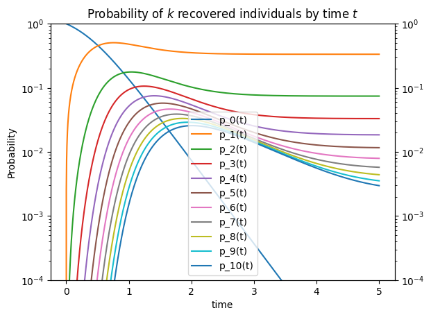
Assume \(\beta = 2\), \(\gamma =1\). Once you have entered the equation for \(\frac{\partial}{\partial t} \Omega(z,t)\) below, the code will solve that equation at each point \(z_m=e^{2 i m\pi/M}\) for \(m = 0, 1, 2, \ldots, M-1\) using an integration method from scipy. Then it performs the equivalent of the Cauchy integral described in Section 1.10 (it actually uses the Fast Fourier Transform) to find the time-dependent coefficients of \(z^\ell\) in the expansion of \(\Omega(z,t)\). You should be able to edit this and run the code in your browser using the “binder” or “live code” links in the ‘rocket’ logo at the top of this page.

Solution (a)

\[ \frac{\partial}{\partial t} \Omega(z,t) = (\beta+\gamma)\left(\frac{\beta}{\beta+\gamma}(\Omega(z,t)^2) + \frac{\gamma}{\beta+\gamma} z - \Omega(z,t)\right) \]

(b) Under the assumptions we have made, it can be shown (not here) that the probability an ~~epidemic~~ outbreak dies out after exactly \(\ell\) infections is \(\frac{1}{\ell} \frac{\mathcal{R}_0^{\ell-1}}{(\mathcal{R}_0+1)^{2\ell-1}} \binom{2\ell-2}{\ell-1}\) where \(\mathcal{R}_0 = \beta/\gamma\). Calculate these for \(\ell = \)0, \(1, 2, 3\) for \(\beta=2\), \(\gamma=1\) and explain the plots created by the code below in terms of these probabilities. Why do some of the probabilities rise and then fall?

Solution (b)

We find \(\mathcal{R}_0 = 2\). So the formula is

\[ \mathbb{P}[\ell \text{ infections}] = \frac{1}{\ell} \frac{2^{\ell-1}}{3^{2\ell-1}} \binom{2\ell-2}{\ell-1} \]

We find:

\(\ell=0\):

The probability must be zero because it is assumed it starts with one infection.

\(\ell=1\):

\[ 1 \frac{2^0}{3} \binom{0}{0} = 2/3 \]

\(\ell=2\):

\[ \frac{1}{2} \frac{2}{3^3} \binom{2}{1} = \frac{2}{9} \]

\(\ell=3\):

\[ \frac{1}{3} \frac{2}{3^5} \binom{4}{2} = \frac{2^2}{3^5} \]

The asymptotes at large \(t\) correspond to these values. At early times, there are more states with a given number recovered, but then more recoveries occur.

from scipy.integrate import solve_ivp
import numpy as np
import matplotlib.pyplot as plt

def dOmega_dt(t, y, beta, gamma, theta):
    """
    Right-hand side of the ODE system.

    We solve for the real and imaginary parts of Omega at each point e^{2 pi i m/M} separately,
    because scipy integrators work with real-valued vectors.

    Parameters
    ----------
    t : float
        Time (not used explicitly here, since the system is autonomous).
    y : ndarray, shape (2M,)
        Current state:
        y = [Re(Omega_1), Re(Omega_2), ..., Re(Omega_M), Im(Omega_1), Im(Omega_2), ..., Im(Omega_M)]
        or equivalently:
        y[0:M]   = Re([Omega_1,...,Omega_M])
        y[M:2M]  = Im([Omega_1,...,Omega_M])
    beta, gamma : float
        Model parameters.
    theta : [0, 1*2pi/M, 2*2pi/M, ..., (M-1)*2pi/M]
           z will become R*exp(i*theta)
    """

    M = theta.size

    # Reconstruct complex Omega from real and imaginary parts
    Omega_real= y[:M]          # real parts
    Omega_imag = y[M:]          # imaginary parts
    Omega = Omega_real + 1j * Omega_imag  #'1j' is the way to denote the square root of -1 

    # Compute z = exp(i*theta)
    z = np.exp(1j * theta)

    ###############################################
    ###############################################
    ####                                       ####
    ####        Fill in Function Here          ####
    ####         (use z insead of x)           ####
    ####                                       ####
    ####                                       ####
    ####     for example, if you had found     ####
    ####   dOmega/dt = 2z^2- Omega^2 + beta    ####
    ####     then set make the line below      ####
    #### dOmega_dt = 2*z**2 - Omega**2 + beta  ####
    ####                                       ####
    ####                                       ####
    dOmega_dt = # YOUR CODE HERE
    ####                                       ####
    ####                                       ####
    ###############################################
    ###############################################


    # Return derivatives as a real vector
    return np.concatenate([dOmega_dt.real, dOmega_dt.imag])


beta = 2
gamma = 1
ell_max = 10
M = 1024

m = np.arange(M) #m = [0, 1, 2, ..., M-1]
# Angles theta = 2*pi*m/M for m=0,...,M-1
theta = 2 * np.pi * m / M

Omega0 = np.ones(M, dtype=complex)
y0 = np.r_[Omega0.real, Omega0.imag]

t_span = (0.0, 5.0)
t_eval = np.linspace(*t_span, 2001)

sol = solve_ivp(dOmega_dt, t_span, y0, t_eval=t_eval, args=(beta, gamma, theta),
                rtol=1e-9, atol=1e-12)

Omega = sol.y[:M].T + 1j*sol.y[M:].T          # (Nt, M)

c = np.fft.fft(Omega, axis=1) / M             # c[:,ell] ≈ p_ell(t)
p  = c[:, :ell_max+1]

for k in range(ell_max+1):
    plt.plot(sol.t, p[:,k].real, label=f'p_{k}(t)')
plt.yscale('log')
plt.ylim(10**(-4),1)
plt.xlabel('time')
plt.ylabel('Probability')
plt.title('Probability of $k$ recovered individuals by time $t$')
plt.legend(loc = 'lower center')
ax1 = plt.gca()
ax2 = ax1.twinx()
ax2.set_yscale('log')
ax2.set_ylim(10**(-4),1)
plt.show()

../../_images/6457ab731541031dcdc2feae71ae7f3ae8f8e1799ffdb44f70063fc632dbddab.png